AI Agent Observability Interview Prep
AI agent observability interview prep: span trees, OpenTelemetry GenAI conventions, production drift types, sampling strategy, and tool selection for senior engineers.
Quick answer
Observability for AI agents is the practice of making agent behavior transparent and debuggable through structured traces, metrics, logs, and drift detectors.
Production AI agents fail in ways that are hard to reproduce and expensive to diagnose without observability.
Editorial review
Written by
CompoundLearn editorial team
Wireless / RF / hardware engineering
Reviewed by
CompoundLearn editorial team
Wireless / RF / hardware engineering
Last reviewed
Built from curated topic maps, editorial validation, and subject-matter review so the page stays aligned with the interview intent and the current content pipeline.
Key points
- AI agent observability makes loop behavior debuggable through structured traces, metrics, logs, and drift detectors, turning a vague weird answer into a traceable causal chain.
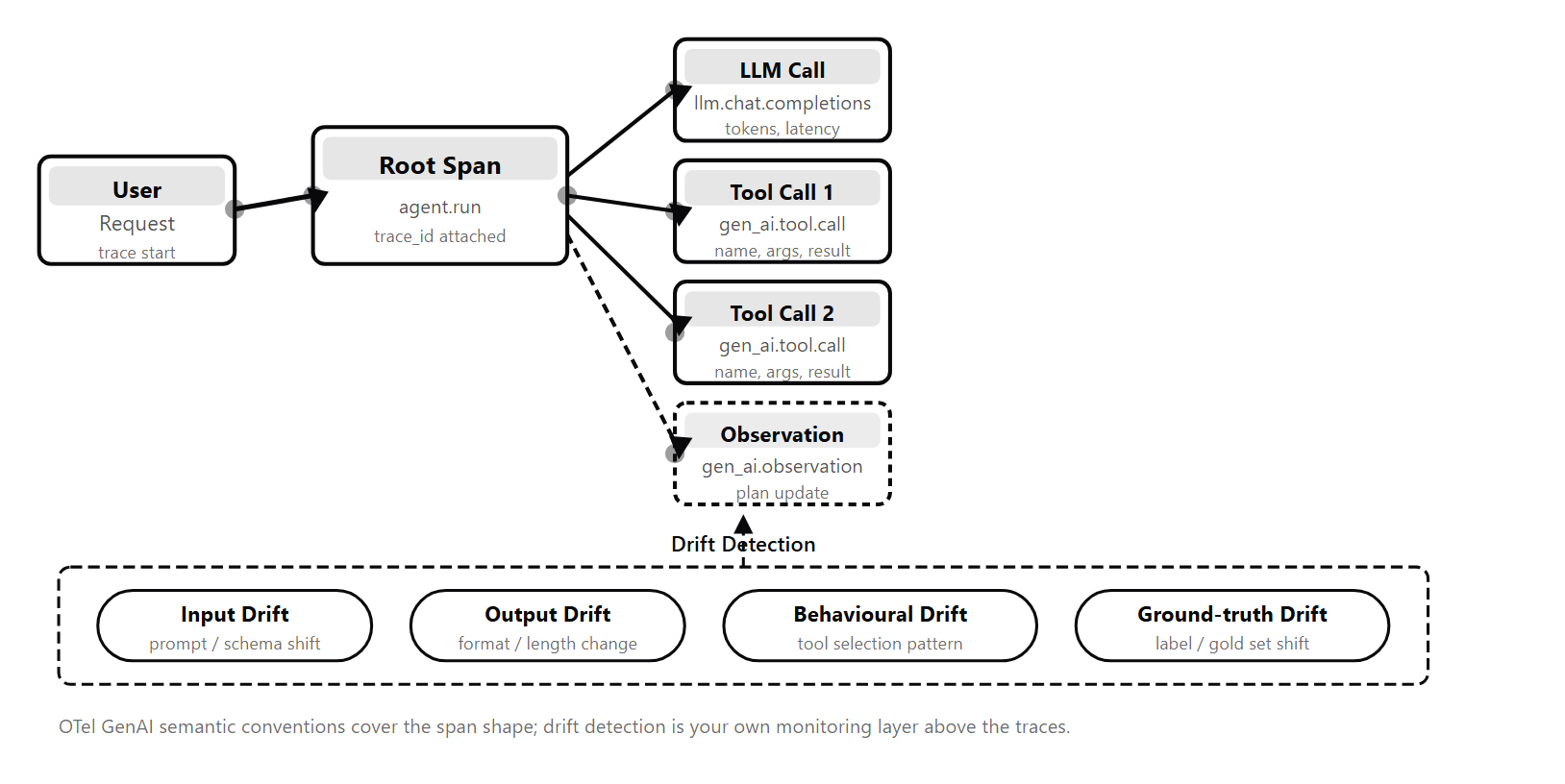
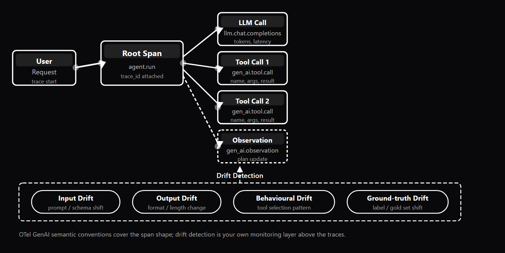
- The span tree, not the log line, is the right unit: a root span (the user request) with child spans for each model reasoning step and leaf spans for each tool call, recording input, output, tokens, cost, and errors.
- Adopting the OpenTelemetry GenAI semantic conventions makes backends (Phoenix, Langfuse, Weave, Datadog, Honeycomb) interchangeable — switching is a config change, not an instrumentation rewrite.
- Production agents show four drift types, each needing a different detector: input drift (embedding centroid), output drift (output distribution), score drift (judge-model shift), and cost/latency drift (rolling-mean ratio).
- Score drift is the silent failure mode — after a judge-model upgrade, identical outputs receive different scores and quality appears to improve when nothing actually changed.
- Always capture 100 percent of errors and high-latency traces (uniform 5 percent sampling misses most rare failures), redact PII at the SDK boundary, and use the trace ID as the join key to evals and the HITL queue.
What it is
Observability for AI agents is the practice of making agent behavior transparent and debuggable through structured traces, metrics, logs, and drift detectors. Because agents run loops — plan, act, observe, replan — a single user request can trigger dozens of internal steps, each of which can fail in a different way. Without observability, "the chatbot gave a weird answer" is guesswork. With it, the same sentence becomes a query: retrieve the trace ID, open the root span, follow the child spans, find the step where the calculation diverged. The span tree is the correct unit of observability for agents, not the log line. A span tree captures the full causal chain: the root span is the user request; child spans are the model reasoning steps; leaf spans are the individual tool calls. Each span records its start time, duration, input, output, token counts, cost, and error state. The canonical span attributes come from the OpenTelemetry GenAI semantic conventions — a vendor-neutral specification for attributes like gen_ai.system, gen_ai.request.model, gen_ai.usage.input_tokens, and gen_ai.response.finish_reasons. Tools that adopt the convention (Phoenix, Langfuse, Weave, OpenLLMetry, Datadog, Honeycomb) are interchangeable; switching backends becomes a configuration change rather than an instrumentation rewrite. Traces serve a second purpose beyond debugging: they are the substrate for the meta-layer of any production agent system. The eval harness replays traces against new model versions to measure regressions. The evaluation-driven improvement loop mines traces for failed cases and proposes prompt improvements. The drift detector queries trace metadata for distribution shifts. The HITL queue pulls low-confidence traces from the trace store for human review. Without trace storage, none of these components have data to work with. Production agent systems exhibit four distinct types of drift that observability must detect. Input drift occurs when the query distribution shifts — new topics, languages, or phrasings — measured via embedding-centroid distance between time windows. Output drift occurs when model outputs change without an obvious cause, often after a silent model-version upgrade — measured via output-embedding distance and length/token distributions. Score drift occurs when the LLM-judge starts scoring differently following a judge-model upgrade, so identical outputs receive different scores — measured by tracking per-rubric-dimension distributions against a held-out validation set. Cost/latency drift occurs when per-task costs and latencies creep up, usually from prompt growth — measured via rolling-mean week-over-week ratio. Each drift type maps to a different architectural layer and requires a different detector. OSS tools for tracing include Langfuse (open-source, self-hostable, acquired by ClickHouse in 2026), Phoenix (Arize, OTel-native, strongest drift detection), W&B Weave (integrates with the W&B ML platform), Helicone (proxy-based, lightest-weight integration), and OpenLLMetry (instrumentation layer that exports to any OTel-compatible backend). Specialized drift tools include Phoenix Drift, Evidently AI, WhyLabs (whylogs), NannyML, and Alibi Detect. Case study: a team running a financial-calculation agent at 10,000 requests/hour discovered a 0.4-point score jump after a judge-model upgrade — scores improved without any change to the agent. Without a versioned drift baseline file and a per-rubric-dimension distribution tracker, the team would have falsely concluded quality improved. Score drift is the silent failure mode that no agent team expects until it happens.
Why interviewers ask
Production AI agents fail in ways that are hard to reproduce and expensive to diagnose without observability. The canonical failure mode is "it works in eval but breaks in prod" — and the reason is almost always an observability gap: the team evaluated on a curated set and had no visibility into the specific edge cases that arrived in production. Interviewers probe observability literacy because it separates engineers who have operated agents in production from those who have only built them. The question "how would you debug a production agent that is producing worse answers than it did last week?" requires knowing: (1) how span trees differ from logs, (2) which trace attributes are mandatory for root-cause analysis (model version, prompt version, retriever config, rubric version), (3) how sampling strategy affects your ability to debug rare failures, and (4) how to connect traces to the HITL queue, the eval harness, and the evaluation-driven improvement loop. Strong candidates can describe all four drift types and explain that each requires a different detector — input drift via embedding-centroid distance, output drift via output-embedding distribution, score drift via per-rubric-dimension shift, and cost/latency drift via rolling-mean ratio. They know that score drift is particularly treacherous because it looks like quality improvement. The "silent quality degradation" scenario is the highest-signal interview probe. Weak candidates describe reactive debugging ("I would look at the logs when something breaks"). Strong candidates describe a proactive posture: a continuous eval loop sampling production traces against a rubric-based judge, a versioned drift baseline file, anomaly-boosted sampling that always captures failures at 100%, and version-tagged traces so any regression is attributable to a specific model or prompt deploy. The advanced signal is knowing where OSS tooling has gaps: no OSS tool specifically monitors for judge-drift (when the judge model upgrades and scores shift), embedding-model drift (when the embedding model upgrades and similarity scores shift), or tool-call distribution drift (when the agent suddenly starts using a different tool than it used to). Knowing the gaps is what distinguishes a senior observability engineer from someone who has read the docs.
Common mistakes
The most pervasive mistake is tracing only the LLM call — capturing the prompt and the response — while ignoring the tool execution spans in between. When an agent fails, the root cause is usually in a tool call: the tool returned an error the agent was not designed to handle, or the tool returned a valid result that was misinterpreted in synthesis. Without tool-level spans, these failures are invisible. The fix is one root span per agent run with child spans for every LLM call AND every tool call AND every retrieval AND every scoring run. The second common mistake is no version tags on traces. A regression appears. Traces don't record which prompt version or model version was in play at the time. You cannot determine whether the regression coincided with last Tuesday's deploy. Version tags (model version, prompt version, rubric version, agent version, deployment region) are a one-time instrumentation investment that makes "did this regression coincide with the deploy?" answerable in two minutes of dashboard time rather than two hours of guesswork. No drift baseline is the third major gap. Teams set up observability for launch and never establish a reference distribution. Without a versioned baseline file, drift detectors either fire on everything (treating the first day's traffic as "drift") or have no comparison window. The fix is to dedicate the first 1-2 weeks of production to baseline collection before turning drift alerts on. PII in traces is the fourth common mistake — and the one that becomes a compliance incident. User queries contain names, emails, account IDs, and other sensitive data. Trace stores are designed for broad developer access (debugging, on-call, ML engineering) and are architecturally weaker from a data-governance perspective than production databases. The fix is redaction at the SDK boundary — both Langfuse and Phoenix provide hooks for this — before any sensitive data reaches the backend. Other high-frequency pitfalls: random sampling that drops the failures (5% uniform random misses 95% of rare failure modes — always capture 100% of errors and high-latency traces), dashboards with 47 widgets that no one reads (cut to 5-10 per team, each tied to a specific decision), and traces disconnected from evals and the HITL queue (the trace ID should be the join key across all downstream artifacts — eval results, annotations, HITL decisions).
Langfuse vs Phoenix vs W&B Weave vs Helicone — Production Agent Observability Trade-offs
| Tool | Hosting Model | OTel GenAI Support | Drift Detection | HITL / Annotation | Best Fit |
|---|---|---|---|---|---|
| Langfuse | Open-source self-hosted (MIT + EE) or managed cloud; acquired by ClickHouse in 2026 | Full OTel GenAI ingestion; native SDKs for Python and TypeScript | Score-threshold alerts and dataset drift alerts; webhook support for custom detectors | Built-in annotation queues; rubric-based score collection per trace | Best when data-sovereignty matters or you need full control; strong product-analytics view |
| Phoenix (Arize) | Open-source self-hosted (EL 2.0) or Arize cloud; auto-traces LangChain, LlamaIndex, OpenAI, Anthropic | OTel-native; OpenInference conventions aligned with OTel GenAI; strongest trace-to-trace comparison | Phoenix Drift module: embedding-space drift, prediction drift, concept drift over rolling windows | Annotation queues via Arize cloud; open-source requires custom tooling for production queues | Best when drift detection and dataset curation are first-class requirements alongside tracing |
| W&B Weave | Apache-2.0; free tier for small teams; paid for large volume; integrates with W&B experiment tracking | Growing OTel GenAI support; native support for OpenAI, Anthropic, LangChain, DSPy | W&B alert system covers Weave traces; integrates with W&B model registry for version comparison | Feedback collection UI built in; integrates with W&B annotation projects | Best when you are already on W&B for ML experiment tracking and want a unified platform |
| Helicone | Apache-2.0; usage-based pricing on managed cloud; open-source version available | Proxy-based: intercepts any OpenAI-compatible API call; broadest provider support via proxy pattern | Cost spike alerts, latency alerts, error rate monitoring; minimal distribution-drift support | Basic feedback logging; not purpose-built for HITL queues; better suited for cost/latency monitoring | Best as a lightweight cost and latency dashboard when full span-tree tracing is not yet needed |
Sample interview questions
- Why is the span tree — rather than a flat log file — the correct unit for agent observability?
- A. Because span trees use less disk space than flat log files at high volume.
- B. Because the span tree preserves the causal hierarchy of a multi-step run: which LLM call triggered which tool call, and in what sequence — information that flat logs lose. ✓
- C. Because OpenTelemetry only supports span-based exporters, not log exporters.
- D. Because span trees allow you to replay an agent run without calling the underlying model.
Option B is correct. A flat log file records events in time order but loses causality: you cannot tell from a timestamp alone whether a tool call was triggered by a specific LLM output or by some other event. The span tree preserves the parent-child relationship — each child span records its parent span ID — so you can reconstruct the full causal graph: this LLM call (root span) produced this tool call (child span), which returned this result (observation span), which led to this replanning step. For debugging a multi-step agent run, this causal structure is essential. Option A is wrong. Storage size is not the reason to prefer spans. Spans and their metadata are often larger than equivalent flat log entries because they carry structured attributes (gen_ai.usage.input_tokens, gen_ai.tool.call.name, gen_ai.system, etc.). Option C is wrong. OpenTelemetry supports multiple signal types: traces (spans), logs, and metrics. The choice of spans for agent tracing is semantic, not a technical limitation of the SDK. Option D is wrong. Span trees do not enable replay — they record what happened. Replay requires separate infrastructure (e.g., storing inputs and deterministic seeds). Spans are for observation, not reproduction. Production reality: Langfuse, Phoenix (Arize), and W&B Weave all ingest OpenTelemetry GenAI spans. Wire your agent to emit spans before the first production session; retrofitting after incidents is painful.
- Using a four-drift framing for production agent systems, which option correctly names all four drift types and their typical measurement approach?
- A. Model drift, data drift, concept drift, and distribution drift — all measured by retraining loss.
- B. Input drift (embedding centroid distance), output drift (output-embedding distance and length distributions), score drift (per-rubric-dimension distribution vs validation set), and cost/latency drift (per-task cost and p50/p95 latency over time). ✓
- C. Latency drift, cost drift, accuracy drift, and throughput drift — all measured by SLA dashboards.
- D. Retrieval drift, generation drift, evaluation drift, and deployment drift — measured by A/B tests.
Option B is correct. Production agent systems exhibit four distinct drift types, each requiring a different measurement strategy: (1) Input drift — the distribution of user queries shifts (new topics, phrasings, languages); measured via embedding-centroid distance between time windows, with an alert at cosine distance > 0.15; (2) Output drift — model outputs change without an obvious cause, often after a silent model-version upgrade; measured via output-embedding distance and length/token distributions, with alerts on KS-test significance; (3) Score drift — the LLM-judge starts scoring differently after a judge-model upgrade, so identical outputs receive different scores; measured by tracking per-rubric-dimension score distributions against a held-out validation set, with an alert when the mean shifts by more than 0.2; (4) Cost/latency drift — per-task costs and latencies creep up, usually due to prompt growth (more retrieved chunks, longer tool histories); measured via rolling-mean week-over-week ratio, with an alert at > 1.2. Option A is wrong. Model drift, data drift, concept drift, and distribution drift are terms from the traditional supervised-ML literature. They do not map cleanly to agent-specific observability, which has richer causality structures (judge-model upgrades, prompt growth) that this taxonomy cannot distinguish. Option C is wrong. Latency, cost, accuracy, and throughput are operational metrics, not drift types. Drift specifically refers to distributional shifts over time — the taxonomy in Option B explains the cause and measurement method for each. Option D is wrong. Retrieval, generation, evaluation, and deployment drift are not the standard categories in the observability literature and conflate distinct concerns. Production reality: each drift type maps to a different architectural layer — input (knowledge layer), output (runtime layer), score (quality layer), cost/latency (meta layer). A single dashboard covering all four is the minimum viable observability posture.
- You are operating an agent at 10,000 requests per hour. Tracing every span at full detail will cost $800/month in storage. How do you set a sampling strategy?
- A. Sample all traces at 100% because any missed trace could hide a critical bug.
- B. Sample at 1% uniformly at random, accepting that rare failures will never appear in traces.
- C. Use anomaly-boosted sampling: a low base rate (e.g., 5-20%) for routine traffic, but always capture 100% of traces that contain errors, high cost, or exceed latency thresholds. ✓
- D. Disable sampling entirely and compress logs to reduce storage costs instead.
Option C is correct. The production-standard strategy is anomaly-boosted sampling: a 5-20% base rate for routine successful traces, combined with always-on capture for traces that indicate interesting events — errors (any span with error=true), high token cost (total cost > threshold), anomalous step counts, or latency outliers. This gives full diagnostic coverage for failures at a fraction of the storage cost, while still capturing a representative sample of healthy traffic for trend analysis and drift baseline computation. Option A is wrong. 100% sampling at high volume is financially unsustainable — the $800/month figure in the question is the cost of doing exactly this. The diagnostic value of the 10,000th trace of a successful routine request is near zero. Option B is wrong. Uniform 1% random sampling is likely to drop the failures you most need to debug. If failures occur at 0.5% of requests, a 1% sample captures only about half of them — insufficient for root-cause analysis. The key fix is always capturing failures, which Option B does not do. Option D is wrong. Compression reduces storage cost but does not change sampling semantics — you still pay to ingest and process every span before compression. Compression is a complementary optimization, not a substitute for a sampling strategy. Production reality: most production systems run 5-20% base-rate sampling with anomaly-driven boost (sample more when error rate or latency spikes). OpenTelemetry supports both head-based and tail-based sampling; for agents, tail-based is preferred because sampling decisions are made after the trace is complete, enabling error-based always-on capture.
- Your team is building a LangGraph-based agent pipeline. When choosing between LangSmith, Langfuse, and Phoenix (Arize) for observability, which criterion most accurately differentiates them for this use case?
- A. LangSmith, Langfuse, and Phoenix are functionally identical for LangGraph pipelines.
- B. LangSmith has the deepest native LangGraph integration (same vendor), Langfuse is the best open-source self-hostable option (acquired by ClickHouse in 2026), and Phoenix adds strong drift detection and dataset-curation workflows on top of OpenTelemetry-native tracing. ✓
- C. Phoenix is the only tool that supports OpenTelemetry; LangSmith and Langfuse use proprietary trace formats.
- D. Langfuse only supports Python agents; LangSmith supports TypeScript; Phoenix supports both.
Option B is correct. The tools have real differentiation: LangSmith is built by the LangChain team and has the deepest native integration with LangGraph — tracing automatically propagates to LangSmith without manual instrumentation, and its dataset-curation tools are optimized for LangChain object shapes. Langfuse is open-source, self-hostable (critical for data-sovereignty requirements), and was acquired by ClickHouse in 2026, which deepens its analytics capabilities; it is the strongest choice when full control over trace data is a constraint. Phoenix (from Arize AI) is OpenTelemetry-native with a strong drift-detection layer — embedding-space drift, prediction drift, and concept drift over rolling windows — making it the best single tool when monitoring for distribution shift is a primary production concern. Option A is wrong. The tools have meaningfully different strengths, hosting models, and integration depths. Treating them as identical leads to a suboptimal observability stack. Option C is wrong. All three tools support OpenTelemetry (OTel) trace ingestion. Phoenix is particularly OTel-native (auto-traces LangChain, LlamaIndex, OpenAI, Anthropic), but Langfuse and LangSmith also support OTel. The differentiator is ecosystem fit and feature depth, not OTel compatibility. Option D is wrong. All three tools support both Python and TypeScript SDKs. The language-restriction claim is false. Production reality: for a LangGraph agent at scale where data must stay in-house, the standard choice is either LangSmith (if vendor lock-in is acceptable) or Langfuse (if self-hosting is required). Add Phoenix's drift detection layer if you have a dedicated ML observability team and distribution-shift monitoring is a first-class concern.
- How do you detect that an agent's output quality has silently degraded in production without explicit user feedback?
- A. Monitor token usage per request — if tokens increase, quality is degrading.
- B. Set up continuous eval on production traces: sample live traces, run them through the same rubric-based LLM-judge used in pre-deployment eval, and alert when the rolling-average score drops below a statistically significant threshold versus the baseline. ✓
- C. Check model version in the API response headers — if the provider upgraded the model, quality may have changed.
- D. Monitor the agent's step count — more steps always indicate worse quality.
Option B is correct. Silent quality degradation without user feedback requires a continuous eval loop on production traffic: (1) sample a percentage of live production traces (5-20%), (2) feed each sampled output through the same rubric-based LLM-judge or scorer used in pre-deployment evaluation, (3) track the rolling-average score over a configurable window, and (4) alert when the score drops below a statistically significant threshold compared to the stored baseline. This is the "continuous eval on production" pattern — it detects model drift, score drift after judge-model upgrades, prompt regression, and knowledge staleness before they accumulate into visible user complaints. Tools like Langfuse and Phoenix support this pattern with online evaluation pipelines. Option A is wrong. Token usage is a cost/latency signal, not a quality signal. An agent can produce more tokens (longer explanations) while improving quality, or produce fewer tokens while degrading. The two metrics are not correlated. Option C is wrong. Monitoring model version tells you that the model changed, not whether quality changed. Model upgrades sometimes improve quality and sometimes introduce regressions. You still need to measure actual output quality — and a silent model upgrade with no version-tag on traces is itself an observability failure (pitfall 4: no version tags). Option D is wrong. Step count is a cost and efficiency metric, not a quality proxy. An agent might solve a problem correctly in 15 steps when 5 would suffice — inefficient but not low quality. Or it might fail in 3 steps — low step count, low quality. Production reality: online eval pipelines that score live traffic against a reference rubric are the industry standard for catching silent quality regressions. Set alert thresholds during initial deployment based on the pre-deployment eval score distribution, and treat the first 1-2 weeks of production as baseline-collection time before turning drift alerts on.
- A user reports that an agent gave a wrong answer on a financial calculation task two days ago. Walk through the trace structure to find root cause. What is the first thing you look at?
- A. The model version used for that specific request, to check if a model upgrade caused the issue.
- B. The root span for that user session: find the trace ID from the error log, open the root span, then follow the child spans to the first step where the intermediate result diverged from the expected value. ✓
- C. The aggregate error rate for the past two days to determine if this was an isolated incident.
- D. The system prompt in effect at the time of the request, to check if a prompt deployment changed the agent's behavior.
Option B is correct. The correct diagnostic sequence is: (1) retrieve the trace ID for that specific user session (from your logging or session ID linkage — the trace ID is the join key across all downstream artifacts), (2) open the root span for that trace in your observability tool, (3) expand the child spans in chronological order, (4) find the first span where the intermediate calculation or tool result diverged from the expected value. This gives you exact reproduction: what input the model received at each step, what tool was called with what arguments, and what the tool returned. If the calculation error is in a tool span, the bug is in the tool. If the calculation error is in the model's synthesis of a correct tool result, the bug is in the prompt or model behavior. Option A is wrong. Model version is a useful secondary check (and should be tagged on every trace), but you cannot diagnose the root cause from it alone. You need to trace the specific session to find where the error occurred. Option C is wrong. Aggregate error rates tell you the magnitude of the problem, not its cause. A 0.1% error rate on a high-stakes financial task is still unacceptable, and you need the individual trace to diagnose it. Option D is wrong. System prompt audit is relevant if the error pattern suggests prompt-level behavior change, but it is a hypothesis, not the first diagnostic step. You start with the specific trace before forming hypotheses — "debug the weird answer is guesswork without traces; with them, it's a query." Production reality: this workflow — trace ID retrieval, root span expansion, child span traversal — is the standard debugging protocol for agent observability. It only works if span-level tracing, with version tags (model version, prompt version, rubric version), was implemented before the incident.
- Your LLM-judge scores for the same outputs jump from an average of 4.1 to 4.5 between two weeks, without any change to the agent or its prompts. What most likely explains this?
- A. The agents's output quality genuinely improved because of diurnal traffic patterns.
- B. Score drift caused by a judge-model upgrade: the provider silently updated the judge model, making it more lenient on the same rubric dimensions. ✓
- C. Input drift: users started sending shorter, easier queries so the outputs are actually better.
- D. Cost/latency drift: the provider reduced token costs, which let the agent generate longer, higher-quality answers.
Option B is correct. This is a textbook case of score drift: the LLM-judge score distribution shifted — same outputs, higher scores — without a corresponding change in actual output quality. The most common cause is a judge-model upgrade by the provider. When the judge model changes (e.g., from one minor version to another), its scoring behavior changes, producing systematically different scores even on identical inputs. Score drift is distinct from output drift (where the agent's outputs change) and from genuine quality improvement. It is measured by tracking per-rubric-dimension score distributions over time and comparing against a held-out validation set; an alert fires when the mean shifts by more than a configured threshold (e.g., 0.2). Option A is wrong. A jump from 4.1 to 4.5 in two weeks without agent changes is too large and too sudden to explain by traffic-pattern effects, which are gradual and diurnal (daily cycles). A genuine quality improvement would also require a traceable cause. Option C is wrong. Input drift (easier queries) could produce better agent outputs and better scores, but this would be detectable as input drift via embedding-centroid distance checks — and the question specifies no change to the agent. If the agent's behavior is the same, simpler queries would produce qualitatively similar outputs, not a 0.4-point score jump. Option D is wrong. Cost/latency drift (token prices, latency) does not cause quality scores to jump. The judge scores outputs, not cost efficiency. Production reality: score drift is a known blind spot — no OSS tool specifically monitors for judge-model-upgrade-induced score shifts. The practical defense is to keep a versioned set of validation outputs with known reference scores and compare live judge scores against that set whenever an alert fires.
- Which of the following is the correct sequence for establishing a drift baseline before going live with a production agent?
- A. Turn drift alerts on immediately at launch, then tune thresholds based on false positives over the next month.
- B. Collect a representative sample of queries, outputs, scores, and latencies during the first 1-2 weeks of production; store it as a versioned baseline file; then enable drift alerts that compare subsequent windows against the baseline. ✓
- C. Use the evaluation set from pre-deployment testing as the drift baseline, since it already represents the expected distribution.
- D. Set static alert thresholds (e.g., score < 3.5) and treat any trace below the threshold as drift.
Option B is correct. The standard practice is: (1) dedicate the first 1-2 weeks of production to baseline collection — gathering a representative sample of live queries, model outputs, LLM-judge scores, and latencies; (2) store this as a versioned baseline file under version control; (3) only then enable drift detectors that compare subsequent rolling windows against the baseline. Without a production baseline, drift detectors either fire on everything (treating the first day's traffic as "drift" from nothing) or on nothing (because the comparison window is empty). The baseline changes only by deliberate decision, so any divergence is a genuine signal. Option A is wrong. Turning drift alerts on immediately at launch and tuning thresholds retroactively leads to alert fatigue: the first weeks of traffic are noisy and non-representative, so thresholds tuned on them will be wrong. Start collecting, then alert. Option C is wrong. The pre-deployment evaluation set is curated and often not representative of the live query distribution — it is deliberately designed to cover edge cases and hard examples. Using it as a drift baseline would make almost all production traffic look like "drift" because real users ask different questions than evaluation authors curate. Option D is wrong. Static score thresholds detect low-quality individual traces, not distributional drift. Drift detection requires a comparison between two distributions (current window vs baseline window), not a per-trace threshold check. A system can have all individual scores above 3.5 while still exhibiting significant score drift. Production reality: the production-checklist item is "version a drift baseline file; compare live distributions against the committed baseline, not against memory." This is a one-time setup cost that prevents months of noisy alerts.
- What is the primary reason to redact PII from trace payloads at the SDK boundary, rather than relying on post-hoc access controls on the trace store?
- A. Redacting at the SDK boundary is faster because it avoids serialization overhead in the trace store.
- B. Trace stores typically have weaker access controls than production databases, and PII that enters the store is hard to selectively delete; redacting before ingestion eliminates the compliance risk at the source. ✓
- C. OpenTelemetry GenAI conventions require PII redaction before spans are emitted.
- D. Post-hoc access controls are not supported by open-source tracing tools like Langfuse and Phoenix.
Option B is correct. Trace stores are observability infrastructure — they are designed for broad accessibility (developers, on-call engineers, ML engineers all query them for debugging). This makes them structurally weaker from a data-governance perspective than production databases, which are typically locked down to application service accounts. User queries, which often contain names, emails, account IDs, and other PII, are the most common trace payload. Once PII enters the trace store, selective deletion is operationally difficult (traces are append-only in most backends) and creates ongoing compliance risk under GDPR, CCPA, and similar regulations. Redacting at the SDK boundary (Langfuse and Phoenix both have hooks for this) eliminates the risk at the source — the trace store never sees the sensitive data. Option A is wrong. Serialization overhead is negligible and not the motivation for PII redaction. The motivation is compliance risk, not performance. Option C is wrong. OpenTelemetry GenAI semantic conventions do not mandate PII redaction — they define attribute names and structures for LLM spans. PII handling is a compliance policy decision, not a convention requirement. Option D is wrong. Both Langfuse and Phoenix support access controls, role-based permissions, and project-level isolation. The point is not that access controls don't exist, but that trace stores are architecturally designed for broad developer access, making PII ingestion a policy risk regardless of controls. Production reality: the production checklist item is "redact PII from trace payloads before they hit the backend; PII in traces is a compliance incident waiting to happen." This is one of the most frequently skipped steps in early-stage agent deployments.
- A new model version is about to be deployed. What observability pattern lets you compare output quality between the old and new versions before exposing users to the new model?
- A. Monitor the new model's error rate in the first hour of production traffic and roll back if it exceeds a threshold.
- B. Run shadow evaluation: serve the previous model version to users while the new version runs in parallel on the same inputs, then compare traces on output quality (rubric scorer or LLM-as-judge on matched pairs), tool-selection agreement, and cost/latency delta. ✓
- C. Compare the pre-deployment eval set scores of both model versions; if the new version scores higher, deploy it.
- D. Use A/B testing: route 50% of traffic to the new model and compare user satisfaction scores after two weeks.
Option B is correct. Shadow evaluation is the production-standard approach for model-version comparison: the previous model version continues serving user-visible traffic while the new version runs in parallel on identical inputs, producing output that is not shown to users. You then compare the two trace sets on three dimensions: (1) output quality — rubric scorer or LLM-as-judge on matched input pairs, giving a direct quality delta; (2) tool-selection agreement — does the new model call the same tools in the same order for the same queries? (significant divergence signals behavioral change); (3) cost/latency delta — tokens per run and wall-clock time per step. Store both trace sets against the same input fingerprints. Phoenix (Arize) has first-class support for trace-to-trace comparison across model versions. Option A is wrong. Monitoring error rate in the first hour of production traffic exposes real users to potential regressions, and a 1-hour window is too short to detect subtle quality degradation. This is a reactive strategy, not a proactive one. Option C is wrong. Pre-deployment eval sets are curated and may not represent the live query distribution. A model that scores well on the curated eval set can still regress on production traffic patterns, especially if the eval set has gone stale (eval rot). Option D is wrong. A/B testing with 50% of traffic and a two-week window exposes a large user cohort to a potentially regressed model for two weeks before you have signal. Shadow evaluation generates the same comparison data with zero user exposure. Production reality: shadow evaluation is the reason version tagging on every trace is non-negotiable. Without model_version and prompt_version tags, the two trace sets cannot be cleanly separated in the observability tool for comparison.
Frequently asked questions
- What is AI agent observability?
- Observability for AI agents is the discipline of recording what a system did so you can answer questions about it later. For agents specifically, it means tracking every step of every run — LLM calls (with model, tokens, cost, finish reason), tool calls (with arguments, output, latency, errors), retrievals (query, top-K results, scores), and scoring runs (rubric version, per-dimension scores, verdict). The right artifact is the span tree, not a flat log file: spans record parent-child relationships, so you can reconstruct causality across the agent loop. Without observability, agent failures are opaque; with it, "the agent failed" becomes "the agent failed at step 4 because the retrieval tool returned an empty result that the planner did not handle gracefully."
- Why is observability critical for agents?
- Agents run loops that are hard to debug. A single user query can trigger 10 or more tool calls across multiple steps. Without structured traces, you cannot tell whether the agent failed because of a bad plan, a broken tool, incorrect data, or a context window overflow. Observability is also the substrate that the eval harness, the evaluation-driven improvement loop, the drift detector, and the HITL queue all depend on — without trace storage, none of these components have data to work with. Silent quality degradation, where the agent slowly worsens across model upgrades or data drift, is only detectable with a continuous eval loop running against a stable baseline.
- What are OTel GenAI semantic conventions?
- OpenTelemetry (OTel) GenAI semantic conventions are a vendor-neutral specification for LLM-application tracing attributes. Key attributes include gen_ai.provider.name (the model provider; gen_ai.system in older spec versions), gen_ai.request.model (the model name), gen_ai.usage.input_tokens and gen_ai.usage.output_tokens (token counts), and gen_ai.response.finish_reasons (why generation stopped). Using these conventions means your traces are queryable in any OTel-compatible backend — Langfuse, Phoenix, Weave, OpenLLMetry, Datadog, Honeycomb, Grafana — without custom parsing. Frameworks like LangChain, LlamaIndex, and the Anthropic SDK emit these attributes natively. Adopting OTel GenAI conventions early means switching backends later is a configuration change rather than an instrumentation rewrite.
- What are the 4 types of production drift in agent systems?
- Input drift: the distribution of user queries shifts (new topics, phrasings, languages), measurable via embedding-centroid distance between time windows. Output drift: the model's outputs change — usually shorter, differently structured, or off-tone — often following a silent model-version upgrade, measurable via output-embedding distance and length distributions. Score drift: the LLM-judge starts scoring differently after a judge-model upgrade, so the same outputs receive higher or lower scores without any change in actual quality, measurable via per-rubric-dimension score distribution against a held-out validation set. Cost/latency drift: per-task costs and p50/p95 latencies creep up — usually because prompts are growing (more retrieved chunks, longer tool histories) — measurable via rolling-mean week-over-week ratio. Each type maps to a different detection strategy and a different architectural layer (knowledge, runtime, quality, meta).
- What should you trace in an agent system?
- For each LLM call: model, temperature, system prompt, messages, tool definitions, output, input/output tokens, cost, latency, finish reason, errors. For each tool call: tool name, arguments, output, latency, errors, retries. For each retrieval: query, top-K results with scores, retrieval method (BM25, vector, hybrid). For each scoring run: rubric version, per-dimension scores, composite verdict. For the agent run as a whole: user ID (or anonymous session), conversation ID, agent version, prompt version, deployment region, total cost, total latency, end state. Spans must have parent-child relationships so you can reconstruct causality. Every trace should also carry version tags — model version, prompt version, rubric version — so regressions are attributable to a specific deploy.
- What is anomaly-boosted sampling in agent tracing?
- Tracing every span of every agent run at full detail is expensive at scale (often more than the LLM bill itself). Anomaly-boosted sampling — also called tail-based sampling — uses a low base rate (5-20%) for routine successful traces, combined with always-on (100%) capture for traces that contain errors, exceed latency thresholds, or fail a quality gate. This means failure cases are fully captured for root-cause analysis, while the healthy majority is sampled for trend analysis and drift baseline computation. Most production systems run 5-20% base-rate sampling with anomaly-driven boost when error rate or latency spikes. Langfuse, Phoenix, and W&B Weave all support configurable sampling policies.
- How does the HITL queue connect to observability?
- The HITL (human-in-the-loop) queue consumes traces directly. Traces tagged with low-confidence scores, errors, or high latency are queued for human review in the same observability UI — Langfuse annotation queues, Phoenix annotation, and Weave feedback collection are all built for this pattern. The annotation feedback flows back to the trace, creating a labeled subset. By aggregating the characteristics of queued traces (which tool failed, which query type triggered escalation), you can detect drift before it shows up in aggregate metrics. A sudden spike in HITL queue volume is often the earliest signal of input drift or a model regression. The trace ID is the join key: every HITL decision, eval result, and annotation references the trace it came from.
- How do you compare traces across model versions?
- Run shadow evaluation: keep the previous model version serving user-visible traffic while the new version runs in parallel on the same inputs. Compare the two trace sets on three dimensions: output quality (rubric scorer or LLM-as-judge on matched input pairs), tool-selection agreement (does the new model call the same tools in the same order?), and cost/latency delta (tokens per run, wall-clock time per step). Store both trace sets against the same input fingerprints — this requires model_version and prompt_version tags on every trace. Phoenix (Arize) has first-class support for trace-to-trace comparison across model versions. Without version tags, the two trace sets cannot be separated for comparison.
- What is the difference between logs, traces, and metrics for agents?
- Logs are text records of events at a point in time — useful for debugging specific errors but hard to query for patterns. Traces are structured, hierarchical records with parent-child span relationships that show causality across the full agent loop — the most valuable observability artifact for multi-step agents because they capture the causal chain across steps. Metrics are aggregated numbers (latency p50/p99, token cost per run, success rate, HITL escalation rate) — useful for dashboards and alerting but not for root-cause analysis. All three are needed: traces answer "what happened in this run?"; metrics answer "what is the same about this run as 1,000 other runs?"; logs fill in point-in-time detail within a span.
- What makes an observability dashboard load-bearing?
- A dashboard is load-bearing if at least one operational decision depends on it per week. A 47-widget "everything" dashboard that teams check monthly is not load-bearing — it is a dashboard nobody reads. Expert practice is purpose-built dashboards: 5-10 widgets each, tied to specific failure modes the team cares about (cost spike, latency regression, score-drift alert, HITL queue volume). Alerts on the 3-5 metrics that actually matter (refusal rate, latency p95, judge-score drift, error rate) do the awareness work; dashboards do the explanation work. A scheduled weekly trace review — reading 2-3 random traces and 2-3 anomaly-flagged traces together — turns observability data into product improvements.
Related topics
Essential AI-Native Skills for AI Agent Observability
Modern engineering work increasingly uses AI tools for design and code review, debugging, documentation, test and testbench generation, and workflow automation. The goal is not to let AI replace engineering judgment — it is to move faster while keeping verification discipline.
- Use AI to explain unfamiliar code, logs, waveforms, datasheets, or test failures.
- Break large problems into small, reviewable steps you can verify independently.
- Ask AI for hypotheses, then validate them against tests, measurements, simulations, or lab data.
- Version-control your analysis scripts, testbenches, and configs — keep changes small and reviewable.
- Document your assumptions, design tradeoffs, and debugging decisions.
- Verify AI output before trusting it: run the checks that fit the domain — unit tests, linters, simulations, or bench/lab measurements.
- Review AI output for correctness, edge cases, and real-world consequences.
Next up: AI Agent Observability practice
The adaptive practice engine is already live for core wireless, RF, and ML domains. AI Agent Observability questions — covering production realities, not just framework syntax — are in active development. Join the early-access list to get them first.