Near-RT RIC vs Non-RT RIC Interview Prep
Near-RT RIC vs Non-RT RIC for interview prep — real-time vs strategic RAN decisions, xApps, rApps, A1 interface, and RAN intelligence control.
Quick answer
The O-RAN RIC is split into two control planes optimized for different decision timescales: Near-Real-Time RIC (<10ms): Makes fast, reactive decisions at edge compute.
Understanding the RIC split is critical for anyone building or deploying Open RAN (see /topics/open-ran-o-ran-interview-prep).
Editorial review
Written by
CompoundLearn editorial team
Wireless / RF / hardware engineering
Reviewed by
CompoundLearn editorial team
Wireless / RF / hardware engineering
Last reviewed
Built from curated topic maps, editorial validation, and subject-matter review so the page stays aligned with the interview intent and the current content pipeline.
What it is
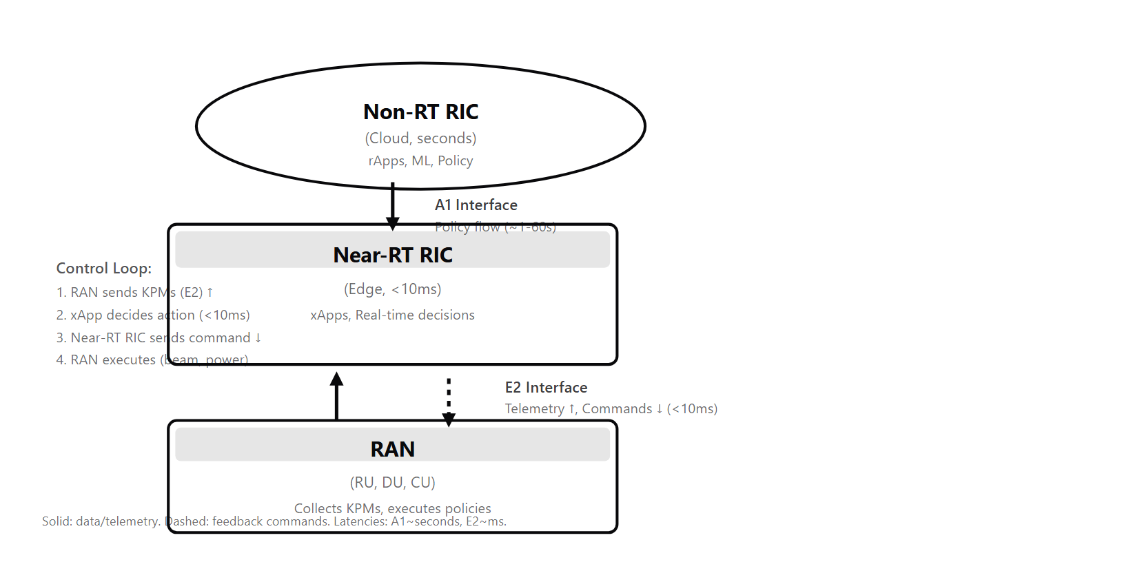
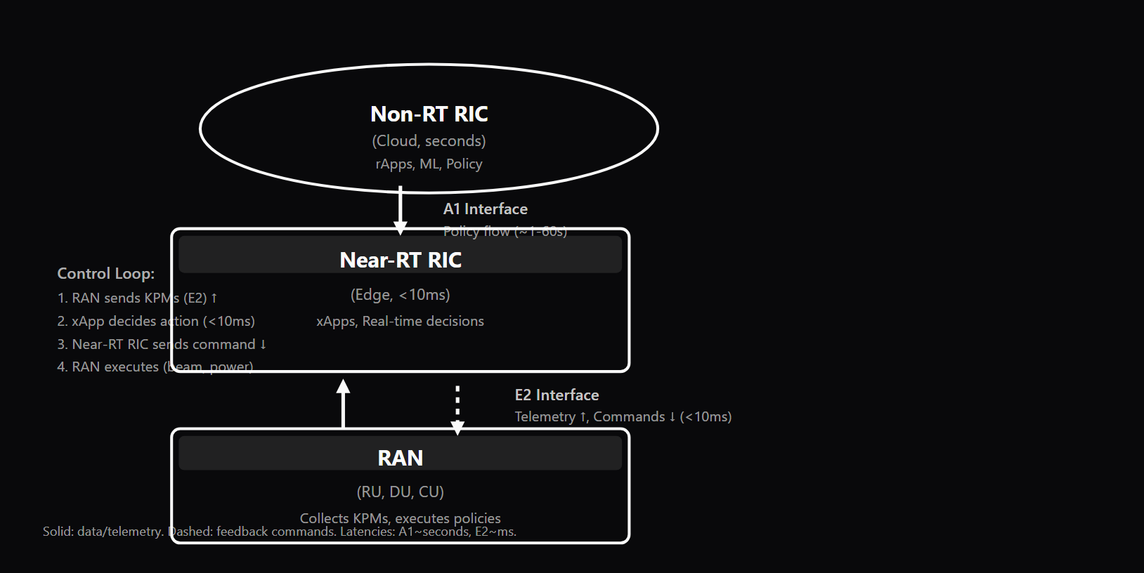
The O-RAN RIC is split into two control planes optimized for different decision timescales: Near-Real-Time RIC (<10ms): Makes fast, reactive decisions at edge compute. Controls beam selection, power allocation, interference mitigation, resource scheduling. Implements xApps that operate at millisecond granularity. Non-Real-Time RIC (seconds to minutes): Makes strategic, compute-intensive decisions in the cloud. Handles policy updates, ML model training, network optimization, load balancing, trend analysis. Implements rApps. The A1 interface connects them: the Non-RT RIC trains models and updates policies, then sends them to the Near-RT RIC, which executes them in real time (see /topics/o-ran-interfaces-a1-e2-o1-o2). This two-tier architecture lets the system be both reactive (fast) and strategic (intelligent).
Why interviewers ask
Understanding the RIC split is critical for anyone building or deploying Open RAN (see /topics/open-ran-o-ran-interview-prep). The challenge is not separate components but their coordination: how does the cloud (Non-RT RIC) train an ML model that improves the edge decisions (Near-RT RIC)? How do you measure whether an rApp is working? Interviewers want engineers who grasp the control plane architecture and can articulate latency-intelligence tradeoffs. Strong candidates can explain why both tiers are necessary, describe how xApps and rApps differ (see /topics/xapps-rapps-ran-intelligence), discuss the A1 policy protocol, and outline how to measure RIC effectiveness (KPI improvement, latency, convergence time for model updates).
Common mistakes
The most common mistake is treating the RIC as a single entity instead of understanding the two-tier split and why it exists. Another gap: confusing xApps with rApps or assuming xApps are just "faster rApps" (the difference is architectural, not just speed). Other pitfalls: not understanding that xApps are deterministic/rule-based while rApps can be ML-based, assuming A1 policy updates are instantaneous (they have convergence time), and missing the fact that the Near-RT RIC still needs local heuristics even with A1 guidance.
Near-RT RIC vs Non-RT RIC — Decision Tiering
| Decision Tier | Latency Budget | Data Rate Handling | Compute Model | Primary Role |
|---|---|---|---|---|
| Near-RT RIC | Sub-10ms (typically 1-5ms per decision cycle) | Real-time KPMs (SINR, power, interference every 100-500ms) | Edge compute; stateless or lightly stateful xApps with rule-based logic | Reactive control: beam steering, power allocation, interference mitigation, per-slice scheduling |
| Non-RT RIC | Seconds to minutes (10s to 1000s of seconds per decision) | Aggregated KPMs, traffic history, model training data (sampled every 10s-1hr) | Cloud compute; stateful rApps with ML models, policy engines, optimization algorithms | Strategic control: policy updates, traffic prediction, load balancing across cells, long-term ML model training |
Sample interview questions
- What is the fundamental architectural reason for splitting the RIC into Near-RT and Non-RT tiers rather than using a single monolithic RIC?
- A. The split is arbitrary; a monolithic RIC would work equally well for all O-RAN deployments
- B. Different RAN decisions operate on fundamentally different timescales with conflicting resource requirements: real-time control (<10ms) demands low-latency edge compute, while strategic optimization (minutes to hours) requires compute-intensive ML and large historical datasets. Separating them allows each tier to be optimized for its workload ✓
- C. The Non-RT RIC is redundant and is rarely used in practice; the Near-RT RIC can handle all decisions
- D. The split forces multivendor compliance and has no technical benefit
Option B captures the core architectural insight. Here's why the split is essential: A Near-RT decision (e.g., beam steering) must execute within ~5 milliseconds of observing the radio condition. To achieve this latency, the RIC must run at edge compute (physically close to the DU), use pre-computed or simple heuristic algorithms (not heavy ML inference), and avoid network round-trips to distant cloud infrastructure. Trying to run this on cloud compute in a far-away data center introduces network latency alone (10-50ms), making sub-10ms decisions impossible. A Non-RT decision (e.g., training an interference prediction model) requires hours of historical data aggregation, matrix operations on GPUs, and iterative algorithm refinement. Trying to run this on edge compute (with limited CPUs and memory) wastes money and fails to leverage the compute scale available in cloud data centers. Also, the Non-RT RIC benefits from running in a cloud-native environment (Kubernetes, persistent databases) that is expensive to replicate at the edge. The A1 interface bridges them: the Non-RT RIC trains a model in the cloud (e.g., "interference typically peaks at 3 PM"), then sends a compact policy to the Near-RT RIC (e.g., "reduce TX power after 2:45 PM to prevent interference at 3 PM"). The Near-RT RIC executes this policy in real time. Option A misses this fundamental mismatch. Option C is factually wrong: the Non-RT RIC is essential for strategic optimization. Option D inverts cause and effect: the split is technical, not a multivendor requirement (though it enables multivendor by allowing vendors to provide different components at each tier).
- An xApp in the Near-RT RIC runs once every 10 milliseconds and adjusts transmit power to maintain a SINR target of 8 dB. A rApp in the Non-RT RIC trains an ML model every hour to predict traffic peaks and recommend power scaling policies. If the ML model predicts a traffic peak at 3 PM and the rApp sends an A1 policy update, how long does it typically take for this policy to affect actual cell power levels?
- A. Less than 1 millisecond because the A1 interface is real-time
- B. The policy affects the next xApp decision cycle (10-100ms) after the policy is parsed, but the xApp may take additional time to apply the policy (hysteresis, validation), so effective convergence is ~100ms to 1 second ✓
- C. Several hours because the Non-RT RIC is slow
- D. The policy update is lost because the Near-RT RIC and Non-RT RIC are asynchronous
Option B is pragmatically correct. Here's the sequence: 1. Non-RT RIC rApp generates the A1 policy at, say, 2:55 PM: "Apply 20% TX power reduction starting 3 PM; revert at 4 PM." 2. The policy is serialized and sent over the A1 interface to the Near-RT RIC. A1 is typically reliable but not real-time; it might take 100-500ms to reach the Near-RT RIC instance(s). 3. The Near-RT RIC receives and validates the policy. If there are multiple Near-RT RIC instances (for redundancy), the update must be replicated (Raft consensus or similar) — another 100-200ms. 4. The xApp running the power control algorithm checks the policy at its next decision cycle. If the xApp runs every 10ms, the policy takes effect within the next 10-100ms. But the xApp typically uses hysteresis (does not flip control parameters on every cycle), so a power reduction policy might ramp in over 5-10 decision cycles = 50-100ms. 5. Effective convergence: from policy generation to cell power actually changing is ~100-500ms in practice. This is NOT a failure — it is by design. The Non-RT RIC operates on minute to hour timescales; a 500ms convergence lag is negligible. But if a designer tried to use A1 policies to react to millisecond-scale events (like a sudden interference spike), they would be disappointed. Option A is too optimistic: A1 is not low-latency. Option C confuses "slow decision process" with "slow convergence time." Option D ignores that A1 is explicitly designed for this asynchronous coupling.
- An xApp in the Near-RT RIC maintains a running estimate of the interference graph (which cells interfere with which neighbors) to optimize beam steering decisions. When the Non-RT RIC detects a topology change (a new cell is added to the network), it must update the Near-RT RIC. Which approach is most robust?
- A. The rApp pushes a complete new interference graph to the xApp via A1, and the xApp immediately replaces its old graph with the new one
- B. The rApp sends only the delta (newly added cell and its interference edges) via A1, and the xApp incrementally updates its graph. This reduces A1 bandwidth, allows the xApp to validate the delta, and ensures the xApp can continue operating on stale data if the A1 update is delayed ✓
- C. The xApp independently learns the new interference graph from KPM data; A1 is not used for topology updates
- D. Topology changes are too rare to require any special handling
Option B reflects best practices in resilient distributed systems. Here's why: **Delta updates:** Sending only the delta (new cell + its interference edges) is much smaller than sending the entire graph. In a large network with thousands of cells, this reduces A1 message size from megabytes to kilobytes. **Validation:** The xApp can validate the delta before applying it. Example: if the rApp claims a new cell is next to cell A, the xApp checks recent KPMs to see if interference metrics align with this claim. Invalid deltas can be logged but not applied, preventing bad topology data from corrupting decisions. **Graceful degradation:** If the A1 update is delayed (network issue, RIC instance overload), the xApp continues using the stale graph. Interference mitigation is slightly suboptimal, but the system does not fail. A full-graph replacement strategy creates brittle coupling: if the replacement is delayed, the xApp has no recent graph and must either fail or fall back to heuristics. **Append-only semantics:** Deltas are more naturally append-only. New cells are added; old cells are not removed (cells are retired, not deleted). This matches the real network lifecycle. Option A is brittle: a delayed full-graph update creates a gap where the xApp operates without topology knowledge. Option C is incomplete: xApps can learn from KPM data, but rApps can detect topology changes much faster (from network management APIs or network logs) than KPMs alone. Option D is unrealistic: in a growing network, topology changes monthly or weekly, not yearly.
- The Near-RT RIC collects Key Performance Measurements (KPMs) from the RAN every 500 milliseconds. An xApp uses these KPMs to adjust the SINR target. A rApp in the Non-RT RIC also uses KPMs (collected every 10 seconds as aggregated statistics) to detect long-term trends. How does KPM granularity affect the decision quality of each?
- A. Granularity does not matter; both xApps and rApps benefit equally from high-frequency KPMs
- B. xApps need high-frequency KPMs (500ms or faster) to react to rapid radio-condition changes and avoid oscillations. rApps need lower-frequency aggregated KPMs (10-60 second windows) to detect trends and filter noise; high-frequency KPMs would introduce too much noise into statistical models ✓
- C. rApps need higher frequency KPMs than xApps because they run ML models that require dense data
- D. Both xApps and rApps should use the same KPM granularity to avoid conflicts
Option B correctly captures the signal-processing tradeoff: **xApps (Near-RT, <10ms decisions):** Radio conditions change fast. SINR can fluctuate ±10 dB within milliseconds due to multipath fading, mobility, or interference. An xApp that adjusts the SINR target needs timely feedback: if it lowered the target expecting interference to rise, it should see that change within ~100-500ms. Delayed KPMs (10-second averages) would not help the xApp learn whether its decision worked. On the flip side, ultra-high-frequency KPMs (1ms snapshots) would be too noisy: random fading fluctuations would trick the xApp into hunting (constantly changing decisions). The "sweet spot" is ~500ms: fast enough to see the effect of decisions, but slow enough to filter out noise. **rApps (Non-RT, minute-to-hour decisions):** rApps detect long-term patterns. "Traffic peaks at 3 PM on weekdays" or "Interference is high near the stadium on game days." These patterns emerge over hours or days of data, not milliseconds. A rApp trying to fit an ML model to 500ms KPMs would overfit to noise and learn spurious patterns. Instead, rApps aggregate KPMs into 10-60 second buckets, removing short-term noise and revealing true trends. An rApp that trained on 500ms KPMs would generate models that are unstable and poor. Bandwidth and processing load are also factors: collecting and transport 500ms KPMs from thousands of cells is expensive. Aggregating to 10-60 second intervals reduces load by 20-120x. Option A misses the core insight: different decision speeds need different data windows. Option C reverses the requirement: ML models need lower-frequency, aggregated data, not higher frequency. Option D ignores that matching granularity to use case is the optimization.
- The Near-RT RIC runs on a cluster of edge servers for redundancy. When one Near-RT RIC instance fails, its xApps' internal state (e.g., learned interference patterns, cached channel estimates) may be lost if not persisted. What is the operational consequence of losing xApp state versus losing rApp state in the Non-RT RIC?
- A. Both are equally catastrophic; the entire RAN becomes unavailable
- B. Losing xApp state degrades RAN performance for ~10-60 seconds (until the xApp relearns patterns from KPMs) but the RAN remains operational. Losing rApp state in the Non-RT RIC is less critical because rApps operate on long timescales and can reinitialize from historical KPMs or rerun model training ✓
- C. Losing rApp state is more critical because rApps control immediate RAN decisions
- D. Neither loss matters because the RIC is optional and the RAN can operate without it
Option B is operationally realistic. Here's why: **xApp state loss:** An xApp maintains dynamic state like "interference graph detected from the last 1 minute of KPMs" or "user mobility patterns observed this session." If the xApp is restarted (due to instance failure), it loses this state. However, the xApp can quickly relearn from fresh KPMs: collect 10-60 seconds of new measurements and recompute the interference graph. During this relearning window (~10-60 seconds), the RAN runs on backup heuristics or default policies, resulting in slightly suboptimal beam steering or power allocation. Cell throughput might drop ~5-10%, but the RAN remains functional and users do not notice brief interruptions. After 1 minute, the xApp has relearned and returns to optimal performance. **rApp state loss:** An rApp is trained on hours or days of historical KPMs (e.g., "interference peaks at 3 PM on Fridays; reduce power proactively at 2:45 PM"). If the Non-RT RIC fails, the rApp restarts. But it can reload its ML model from cloud storage (Kubernetes PersistentVolumes) or retrain in minutes from historical KPMs in a database. The retraining is expensive (GPU time, delay) but not urgent: the rApp's decisions take effect over minutes to hours anyway. While the rApp retrains, the Near-RT RIC still operates with last-known policies (A1 policies from before the failure), which is probably adequate. The key difference: xApps are reactive and stateful; losing state creates a brief blind spot. rApps are strategic and can reload state from persistent storage. Option A is overstated: neither failure is catastrophic because xApps have fallback heuristics and rApps have persistent models. Option C reverses priorities: xApps impact immediate control, not rApps. Option D is wrong: the RIC is essential for modern RAN optimization.
- Feedback oscillation can occur when an xApp and rApp conflict: the xApp makes a fast decision (e.g., reduce TX power), the rApp observes the result and sends a policy to increase power, the xApp then increases power again, and the cycle repeats. How can this oscillation be prevented?
- A. Oscillation cannot be prevented; it is an inherent limit of two-tier RIC architecture
- B. Implement hysteresis in the xApp (require a margin before changing power again), give rApps sufficient measurement windows to detect real trends, enforce rate limits on A1 policy updates, and validate the feedback loop with simulation before deployment ✓
- C. Run all decisions in the Near-RT RIC and eliminate the Non-RT RIC
- D. Synchronize xApp and rApp decision cycles so they run at the same frequency
Option B provides practical engineering solutions. Here's each technique: **Hysteresis in the xApp:** Instead of changing power every cycle, require a change only if the metric exceeds a threshold by a margin. Example: "increase TX power only if SINR drops below 5 dB AND stays there for 3 consecutive decision cycles (30ms)." This prevents the xApp from reacting to every noise fluctuation and creating thrashing. **Measurement windows in the rApp:** Instead of updating the A1 policy every minute based on instant metrics, rApps should observe trends over longer windows (e.g., 10 minutes of data). This filters noise and ensures the rApp detects a real trend, not a temporary fluctuation. **Rate limits on A1:** Even if the rApp detects a trend, do not send A1 policy updates faster than once per minute. This ensures the xApp has time to adapt to one policy before the next arrives, preventing whiplash. **Simulation before deployment:** Before deploying an xApp-rApp pair, test them together in a simulation. Feed realistic RAN conditions (channel traces, traffic patterns) to both and verify the feedback loop converges rather than oscillates. Real deployments catch edge cases, but simulation catches the obvious problems. Option A is defeatist: oscillation is a well-known issue in control systems and has standard mitigation. Option C removes the strategic tier and loses intelligence. Option D ignores that the two tiers are optimized for different timescales; forcing the same frequency defeats the architecture.
- A Non-RT RIC rApp detects that a newly deployed ML model improves traffic prediction by 15% (measured on historical data). The rApp sends the model weights to the Near-RT RIC via A1 for the xApps to use in real-time scheduling. Why might the model perform worse in live deployment than in historical testing?
- A. ML models always perform worse in production due to general overfitting
- B. The model may have been trained on historical data that does not reflect current network conditions (concept drift), and live traffic patterns might differ from training data. Also, the model inference latency (milliseconds) in the xApp might be too slow, causing the xApp to use stale predictions. Additionally, the model might assume stationary traffic, but real networks experience seasonal patterns and anomalies ✓
- C. The A1 interface corrupts the model weights during transmission
- D. ML models cannot be used in xApps because xApps must be deterministic
Option B describes real-world challenges when moving ML models from offline evaluation to live systems: **Concept drift:** The model trained on last month's data might not work today if traffic patterns have shifted. Seasonal changes (holidays, school terms), new applications (TikTok trends), or infrastructure changes (new cell added) alter the underlying data distribution. The model is "confident" on historical data but surprised by live data. **Stale predictions:** An xApp runs the ML model once per 10-100ms to predict the next user activity or cell load. But by the time the xApp acts on that prediction (5-10ms later), the ground truth has changed. In a fast-moving system, predictions become stale quickly. A model optimized for offline batch prediction can behave poorly in low-latency online settings. **Traffic anomalies:** The model assumes normal conditions. When a sporting event, disaster, or viral social media moment causes traffic to spike unexpectedly, the model has no pattern to match and produces poor predictions. Robust models need anomaly detection and fallback heuristics, which offline evaluation skips. **Feedback loops in live deployment:** In offline testing, the model outputs a prediction and does not affect the input. In live deployment, the xApp acts on the prediction, which changes the RAN behavior, which changes future traffic, which changes the input to the next prediction. The model is now part of a closed loop and can amplify errors. **Solution:** Deploy the model cautiously (shadow mode: log predictions but do not act on them), monitor live performance against historical benchmarks, and retrain frequently (daily or weekly) with fresh data. Option A is too broad; not all models overfit, and good ML engineering mitigates overfitting. Option C is wrong: A1 is reliable. Option D is false: xApps can certainly use ML-based logic; the constraint is latency, not determinism.
- In a multi-region O-RAN deployment, each region has its own Near-RT RIC instance (for low latency), but all regions share a single cloud-hosted Non-RT RIC. What architectural challenge arises when the Non-RT RIC trains a global ML model and distributes it to multiple regional Near-RT RIC instances?
- A. Multi-region deployment is not possible with the O-RAN split-RIC architecture
- B. The challenge is model staleness: each regional Near-RT RIC receives the model at different times and may interpret global policies differently due to local network variations. Additionally, coordinating A1 policy updates across regions requires synchronization, and regions with different deployment maturity might receive incompatible model versions. Solution: version the models, use gradual rollout with canary deployment, and allow each region to adapt the global model to local conditions ✓
- C. All regions must use identical models; customization is forbidden
- D. Multi-region deployments require separate Non-RT RICs per region to avoid this problem
Option B captures real operational complexity in large-scale O-RAN: **Model staleness:** The Non-RT RIC trains a global model using data from all regions (e.g., "nationwide interference patterns"). It then distributes the model to, say, 5 regional Near-RT RIC instances via A1. But the instances receive it at different times due to network latency and local processing load. Region 1 gets the model 100ms after training; Region 5 gets it 5 seconds later. In the meantime, Region 1 is running the new model, Region 5 is still using the old one. For 5 seconds, the regions are in different states, potentially creating inconsistent RAN behavior (e.g., load-balancing decisions conflict). **Local variation:** A global model trained on nationwide data might not be optimal for regional sub-networks. For example, a model that predicts high traffic at 3 PM works for the main city but fails in rural regions with different traffic patterns. The model might even be harmful if it causes the rural Near-RT RIC to make suboptimal local decisions. **Version mismatch:** If the Non-RT RIC rolls out model version 2.5 while some regions are still on 2.4 (due to delayed A1 delivery or instance failures), regions running different versions might make conflicting decisions. One region's model says "high interference," another says "low"; coordinated interference mitigation fails. **Solution:** - Version the models and tag A1 messages with the model version. - Use canary deployment: roll out the new model to one region first, monitor for 10-30 minutes, then roll out to others. - Allow regions to override or adapt policies locally if they detect conflicts. - Validate model compatibility across versions before deployment. Option A is incorrect: multi-region is standard. Option C is wrong: customization is necessary for performance. Option D is incorrect: a single cloud Non-RT RIC scales better than replicated instances; the challenge is managed, not avoided.
- How does the E2 interface (RAN to Near-RT RIC) differ from the A1 interface (Non-RT RIC to Near-RT RIC) in terms of data flow direction, latency requirements, and information type?
- A. E2 and A1 are functionally identical; the names are different only for standards compliance
- B. E2 is bidirectional (RAN ↔ Near-RT RIC): uploads KPM telemetry to the RIC and downloads control directives to the RAN. E2 latency is <10ms. A1 is unidirectional (Non-RT RIC → Near-RT RIC): carries policy updates and model parameters. A1 latency is relaxed (seconds). E2 carries fine-grained KPM data; A1 carries high-level policies ✓
- C. A1 carries KPMs and E2 carries policies; they are reversed in the diagram
- D. E2 is optional; A1 is the only required interface
Option B clearly delineates the two interfaces, which are fundamentally different: **E2 Interface (RAN ↔ Near-RT RIC):** - Direction: Bidirectional (both control and reporting) - Latency: <10 milliseconds (critical for real-time feedback loops) - Uplink (RAN → RIC): KPM subscriptions and indications. The RIC subscribes to metrics ("send me SINR every 100ms"), and the RAN streams back KPMs. High data rate (~1-10 Mbps per cell) because it carries detailed telemetry. - Downlink (RIC → RAN): Control directives from xApps. Example: "adjust beam angle by +5 degrees" or "set TX power to -10dBm." Lower data rate because commands are sparse. **A1 Interface (Non-RT RIC → Near-RT RIC):** - Direction: Unidirectional (cloud to edge) - Latency: Relaxed (seconds to minutes acceptable) - Content: Policy updates, ML model parameters, configuration changes from rApps. Example: "apply energy-saving policy: reduce power by 10% after 11 PM" or "update load-balancing weights: Region A gets 60%, Region B gets 40%." Very low data rate because policies are sent infrequently and are highly compact (kilobytes). The distinction is crucial: E2 is the nervous system (constant real-time feedback), while A1 is the policy layer (occasional strategic updates). Confusing them misses the fundamental architecture. Option A misses the critical differences in data flow, latency, and semantics. Option C reverses them. Option D is wrong: both are essential for the two-tier RIC to function.
Frequently asked questions
- What is the Near-RT RIC?
- The Near-Real-Time RIC makes decisions with sub-10-millisecond latency: beam selection, power control, resource allocation, interference mitigation. It runs close to the RAN (often edge compute) to meet strict latency budgets.
- What is the Non-RT RIC?
- The Non-Real-Time RIC makes decisions at longer timescales (seconds to minutes): policy updates, ML model training, network optimization strategy, load balancing across cells. It runs in the cloud and updates the Near-RT RIC via the A1 interface.
- Why split the RIC into two?
- Splitting allows the system to optimize for two very different decision speeds. Near-RT decisions must be fast and reactive (beam adjustment every millisecond). Non-RT decisions can be slow, compute-intensive, and strategic (training an ML model to optimize traffic).
- What are xApps and rApps?
- xApps run in the Near-RT RIC and make fast decisions (beam steering, power control). rApps run in the Non-RT RIC and make slower, policy-level decisions. Both use data from the RAN (KPMs — Key Performance Measurements) and the A1 interface connects them.
- What is the A1 interface?
- The A1 interface connects the Non-RT RIC to the Near-RT RIC. It carries policy decisions, ML model parameters, and configuration updates from the Non-RT RIC to guide the Near-RT RIC's fast decisions.
- What are concrete examples of A1 policy decisions?
- An A1 policy might specify: 'Set maximum beam angle to ±30 degrees' (constraining beam steering xApp), or 'Target SINR floor = 5dB; if unachievable, trigger load balancing to adjacent cells' (steering power allocation), or 'Apply radio resource management (RRM) policy: favor low-latency slices on weekday mornings, eMBB on afternoons.' The Non-RT RIC computes these policies from traffic trends, cost optimization, and SLA contracts; it then sends them to the Near-RT RIC's xApp framework, which enforces them in real time.
- What is the KPM collection overhead and how does it affect RIC decisions?
- Key Performance Measurements (KPMs) are RAN metrics (SINR, throughput, latency, cell load, handover counts) that xApps and rApps consume to make decisions. Collecting KPMs adds overhead: each cell samples radio conditions, computes aggregate statistics, and reports them via the E2 interface (typically every 100ms to 1 second). High-frequency KPM collection (10ms intervals) enables more responsive xApps but consumes RAN processing capacity and backhaul bandwidth. Operators tune KPM granularity and sample rate based on the decision speed of their xApps; a beam-steering xApp needs faster KPMs than a load-balancing rApp.
- How long does it take for an A1 policy update to converge across the RAN?
- Policy convergence time depends on the update mechanism. A stateless xApp (e.g., beam angle limits) converges immediately — the next decision cycle applies the new constraint. Stateful xApps (e.g., reinforcement learning agents maintaining internal state) may require several decision cycles to adapt. rApp policy updates (e.g., new ML model weights) typically take seconds to minutes because the Non-RT RIC must validate the model, serialize it, distribute it to one or more Near-RT RIC instances, and wait for all xApps to reload. In clustered deployments with redundant Near-RT RICs, synchronizing state across instances adds latency. Operators must design for eventual consistency, not instantaneous convergence.
- How do xApps and rApps synchronize state during RIC failover?
- State synchronization during failover is a major operational challenge. When a Near-RT RIC instance fails, its xApps' internal state (learned beam patterns, interference graphs, power budgets) may be lost unless explicitly persisted. The O-RAN standard does not mandate state persistence; implementation is vendor-specific. Best practice: xApps store critical state in a shared distributed cache (e.g., Redis) accessible by backup RIC instances. The Non-RT RIC (which is cloud-hosted and can use Kubernetes StatefulSets) inherently persists state, so rApps recover more cleanly. The trade-off is complexity: stateless xApps are simpler but less intelligent; stateful xApps with persistence are harder to debug and require careful consistency protocols.
- What feedback loop stability issues arise when Near-RT and Non-RT RICs interact?
- The feedback loop between xApps and rApps can oscillate if policies and real-time decisions interact poorly. Example: a beam-steering xApp maximizes SINR locally; a load-balancing rApp notices high cell load and shifts traffic to adjacent cells; the xApp responds by steering more beams toward the overloaded neighbor, which rApp then offloads again. Poorly tuned xApp-rApp pairs create hunting behavior. Mitigation: (1) design xApps with hysteresis (only change decisions if metric exceeds threshold by margin), (2) give rApps sufficient measurement windows to detect real trends versus noise, (3) enforce rate limits on policy updates so rApps do not react faster than the RAN can adapt, (4) use simulation to validate the feedback loop before deployment.
Related topics
Essential AI-Native Skills for Near-RT RIC vs Non-RT RIC
Modern engineering work increasingly uses AI tools for design and code review, debugging, documentation, test and testbench generation, and workflow automation. The goal is not to let AI replace engineering judgment — it is to move faster while keeping verification discipline.
- Use AI to explain unfamiliar code, logs, waveforms, datasheets, or test failures.
- Break large problems into small, reviewable steps you can verify independently.
- Ask AI for hypotheses, then validate them against tests, measurements, simulations, or lab data.
- Version-control your analysis scripts, testbenches, and configs — keep changes small and reviewable.
- Document your assumptions, design tradeoffs, and debugging decisions.
- Verify AI output before trusting it: run the checks that fit the domain — unit tests, linters, simulations, or bench/lab measurements.
- Review AI output for correctness, edge cases, and real-world consequences.
Near-RT RIC vs Non-RT RIC — coming to the question bank
The adaptive practice engine is already live for core wireless, RF, and ML systems. Near-RT RIC vs Non-RT RIC isn't covered in the question bank yet — get notified when it's added.