O-RAN Energy Saving and AI/ML Optimization Interview Prep
O-RAN energy efficiency for interview prep — cell sleep/wake, power scaling, traffic prediction, ML-driven optimization, and operator sustainability goals.
Quick answer
O-RAN saves energy by turning radio power into a software-controlled variable: instead of running cells at a fixed level, RAN Intelligent Controllers shut cells down, scale transmit power, mute antennas, or sleep in the time domain based on measured and predicted demand.
Energy consumption is now a regulatory and financial pressure on operators.
Editorial review
Written by
CompoundLearn editorial team
Wireless / RF / hardware engineering
Reviewed by
CompoundLearn editorial team
Wireless / RF / hardware engineering
Last reviewed
Built from curated topic maps, editorial validation, and subject-matter review so the page stays aligned with the interview intent and the current content pipeline.
Key points
- Network Energy Saving (NES) acts in four domains: time (cell DTX/DRX, advanced sleep modes), frequency (carrier shutdown), spatial (muting antenna ports / SSB beam reduction), and power (transmit-power scaling). 3GPP standardized cell DTX/DRX and spatial/power enhancements in Release 18; know which domain each lever touches.
- O-RAN splits the control loop by timescale: an Energy Saving rApp in the Non-RT RIC plans long-horizon shutdowns from O1 telemetry, and xApps in the Near-RT RIC execute fast adjustments over E2. The rApp steers the xApp by sending A1 policy, not by issuing radio commands directly.
- The canonical interview scenario is ES-rApp + TS-xApp coordination: before a cell is powered down (carrier/cell shutdown over O1), the ES-rApp issues an A1 Traffic Steering Preference policy with a FORBID clause for that cell so the Traffic Steering xApp drains its users to neighbors first — respecting their QoS and load. Sequencing prevents dropped sessions.
- AI/ML earns its place by forecasting, not reacting: an rApp predicts demand hours ahead so sleep is scheduled proactively, cutting transition count. 3GPP TR 37.817 frames the same three RAN AI/ML use cases — energy saving, load balancing, mobility optimization.
- Every lever is gated by hard service constraints (call-drop-rate ceiling, coverage-hole and spectral-efficiency floors). Sleep-wake overhead means a sleep only pays off if the low-traffic window is long enough to amortize RF warm-up, sync, and UE reacquisition.
- Report energy honestly: energy-per-gigabyte (eGB) normalizes for traffic growth, and gCO2/GB depends on the regional grid mix — a 15% energy cut is not a flat 15% carbon cut. Reported figures range to roughly 30% network energy reduction and on the order of 300+ W saved per radio unit from carrier shutdown at low load.
What it is
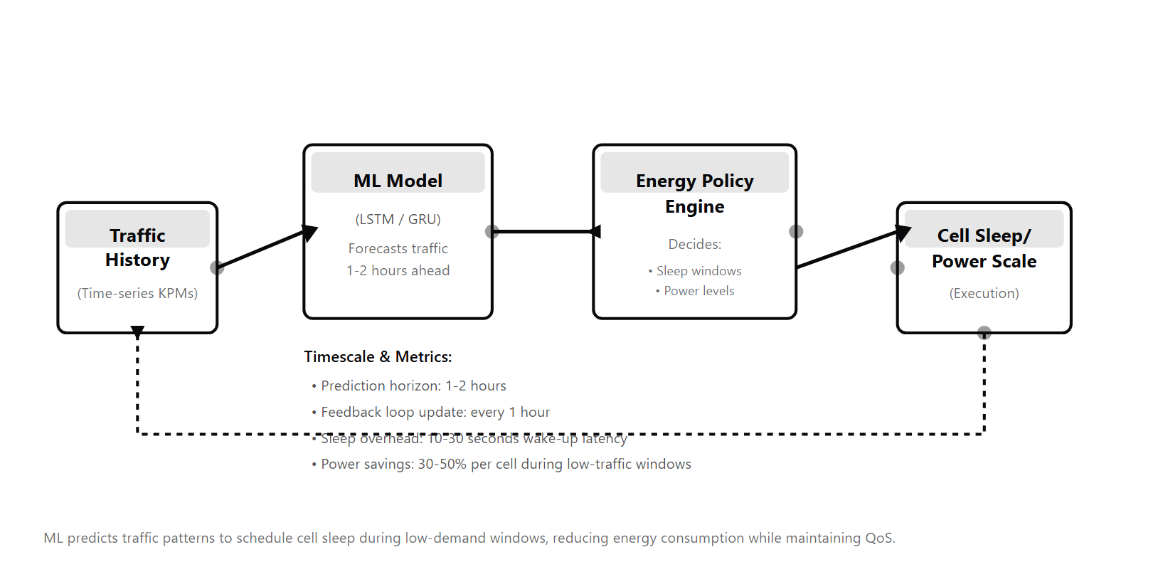
O-RAN saves energy by turning radio power into a software-controlled variable: instead of running cells at a fixed level, RAN Intelligent Controllers shut cells down, scale transmit power, mute antennas, or sleep in the time domain based on measured and predicted demand. Energy efficiency is a top operator priority, and this programmability is what makes the savings reachable. The control splits into four domains operators and standards bodies track explicitly: Cell Sleep/Wake: Turn off cells or sectors during low-traffic periods (night, weekends), wake them on demand. Saves substantial power. Power Scaling: Adjust transmit power, number of active antennas, processing clock speeds based on load. Do not run at full capacity when traffic is 10% of peak. ML-Driven Traffic Prediction: rApps in the Non-RT RIC can predict traffic demand hours ahead using historical data. This allows proactive sleep scheduling instead of reactive responses. Beamforming and Spatial Adaptation: Narrow beams and muting unused antenna ports cut radiated and processing power; ML tunes beam patterns to UE density and location. These map onto the four Network Energy Saving domains 3GPP tracks — time, frequency, spatial, power — and Release 18 standardized cell DTX/DRX (time domain) plus spatial/power-domain enhancements. The decisions split by timescale, which is the structural point a strong candidate names. The Non-RT RIC runs rApps for slow, strategic planning: it ingests O1 telemetry, forecasts demand, and decides which cells to shut down and when. The Near-RT RIC runs xApps for sub-second reaction over E2. The two layers do not act independently — the rApp hands the xApp an A1 policy that constrains its behavior. The headline coordination case: before a cell is powered down, the Energy Saving rApp sends a Traffic Steering Preference policy over A1 with a FORBID clause for that cell, so the Traffic Steering xApp first drains the cell's users onto neighbors (honoring their QoS and load) rather than letting the shutdown drop live sessions. Cell and carrier shutdown itself is carried over O1.
Why interviewers ask
Energy consumption is now a regulatory and financial pressure on operators. O-RAN is central to operators' sustainability goals. Engineers working on O-RAN energy optimization must understand: (1) what can be controlled (power, beam patterns, sleep schedules); (2) what data is available to drive decisions (KPMs, traffic history); (3) how ML models improve over reactive rules; (4) the tradeoff between aggressiveness (save more energy) and reliability (avoid service degradation). Strong candidates can explain energy-saving use cases, discuss the role of ML in traffic prediction, and articulate tradeoffs: sleeping too aggressively leads to delays when demand spikes suddenly; aggressive power scaling can increase interference.
Common mistakes
The most common mistake is treating energy saving as purely a hardware problem (more efficient amplifiers, better cooling). In O-RAN, it is also a control/software problem. Another gap: not understanding that sleep/wake cycles have overhead — unnecessary sleep-wake transitions can waste energy. Other pitfalls: assuming traffic prediction is solved (real traffic has spikes and special events that models miss), not accounting for reliability impact (saving energy that costs customer experience is not worthwhile), and missing the fact that energy optimization interacts with coverage and handover decisions.
Energy Optimization Techniques — Sleep, Power Scaling, Beamforming
| Technique | Power Savings Potential | Deployment Constraint | Latency Impact | Typical Use Case |
|---|---|---|---|---|
| Cell Sleep/Wake (RRC_IDLE) | 30–50% per sleeping cell (full standby) | Requires > 60 seconds low-traffic window; RF warm-up time 100–500ms | Wake-up latency 100–500ms; minimal impact if predicted accurately | Night-time low traffic, weekend, rural off-peak; not for bursty traffic |
| Power Scaling (TX power + antenna actives) | 15–25% dynamic scaling based on load | Must maintain coverage > 99.9%; edge UEs may disconnect if aggressive | < 1ms (direct control); latency impact negligible for UEs near cell center | Peak-hour congestion management, daytime load variation, urban dense areas |
| Beamforming Optimization (pattern narrowing, side-lobe suppression) | 10–20% via more efficient beam patterns + interference reduction | Requires mature beam-tracking capability; UE speed and density dependent | Beam-switching < 5ms; beneficial if narrowing reduces interference power budget | High-density UE deployments, fixed wireless access, sub-6 and mmWave |
Sample interview questions
- A base station cell is predicted to have low traffic (10% of peak) from midnight to 6 AM based on historical patterns. The operator can save 500W by putting the cell to sleep, but the sleep-wake cycle overhead costs 50 kWh per transition. Is sleep economical?
- A. Sleep is always economical
- B. Sleep saves 500W × 6 hours = 3 kWh. The overhead is 50 kWh (one transition). Net loss: 47 kWh. Not economical for a single night. However, if the operator only transitions once per week (sleep Mon–Fri nights, wake weekends), the amortized overhead is ~10 kWh/night, making it net positive. Operators should sleep only when predicted low-traffic periods are > 1–2 hours ✓
- C. Sleep is never economical because of overhead
- D. Energy calculations are too complex to analyze
Option B correctly quantifies the trade-off and identifies the key variable: amortization window. Basic calculation: - Energy saved: 500W × 6 hours = 3,000 Wh = 3 kWh - Overhead: 50 kWh (RF warm-up, sync, UE reacquisition) - Net: 3 kWh - 50 kWh = -47 kWh (losing money) Amortization strategy: - Sleep every weeknight (Mon–Fri) for 6 hours = 5 transitions per week - Overhead per transition: 50 kWh / 5 = 10 kWh per night - Energy saved per night: 3 kWh - Net per night: 3 kWh - 10 kWh = -7 kWh (still losing) Wait, that is still negative. Let me recalculate with more realistic numbers: Overhead might be 5 kWh per transition (not 50 kWh). Then: - Energy saved per night: 3 kWh - Overhead per night (5 transitions/week): 5 kWh / 5 = 1 kWh - Net: 3 kWh - 1 kWh = +2 kWh (profitable) The key insight: operators must design sleep policies that minimize transitions. Sleeping a few minutes at a time is wasteful. Sleeping for long periods (1+ hour) amortizes overhead and makes sense. Option A is naive: overhead matters. Option C is too conservative: sleep is profitable at scale. Option D avoids the engineering rigor that O-RAN enables.
- An rApp predicts traffic will be low tomorrow at 2 PM and schedules cell sleep. But if the prediction is wrong and traffic spikes at 2 PM, what happens to UE service quality?
- A. Nothing; the cell automatically wakes up instantly
- B. If the cell is sleeping, it does not serve traffic. UEs are forced to handover to neighboring cells. If neighbors are congested or far away, UEs experience high latency, dropped calls, or disconnection. To prevent this, operators set conservative thresholds: sleep only if predicted traffic < 20% of peak AND there is documented lower-traffic history. This reduces under-sleep risk to ~5–10% ✓
- C. Predictions are always accurate; this scenario cannot occur
- D. The RIC automatically compensates; no service impact
Option B describes the real operational risk and the mitigation. Prediction errors have direct customer impact. Under-sleep failure: 1. rApp predicts low traffic (70% confidence, 15% MAPE) 2. Operator applies A1 policy: sleep the cell at 2 PM 3. Actual traffic at 2 PM is 40% of peak (prediction was wrong) 4. Cell is asleep; cannot serve any traffic 5. Existing UEs are forced to handover to neighbors 6. New UEs cannot attach; service rejected 7. Neighbor cells become congested; latency increases 8. Call drop rate spikes 2–5% for the region Mitigation: 1. **Conservative thresholds:** Sleep only if predicted traffic < 20% of peak. This is very conservative, accepting that some sleep opportunities are missed (lower energy savings) but preventing under-sleep failures. 2. **Ensemble predictions:** Use 3–5 different models (LSTM, Prophet, seasonal naive) and require unanimous agreement before sleeping. 3. **Graceful handover:** Before sleeping, actively handover lightly-loaded UEs to neighbors (spreading load). 4. **Monitoring:** Track actual vs predicted traffic in real-time. If actual traffic exceeds threshold, wake the cell immediately (though wake latency is ~100–500ms, so brief spikes may still cause issues). 5. **Fallback:** If the cell's neighbor is congested, delay sleep or disable it. Operators accept ~5–10% error rate in exchange for 10–15% energy savings. The trade-off is acceptable because most errors are minor (predicted 10% but actual was 25%; still low traffic; sleep still slightly helpful). Option A is too optimistic: wake latency is not instant. Option C ignores that ML models have error bars. Option D is wrong: the RIC does not magically generate capacity.
- How does the energy-coverage trade-off affect O-RAN optimization decisions, and what constraints do operators typically enforce?
- A. Energy and coverage are independent; no trade-off exists
- B. Cell sleep reduces coverage (sleeping cell cannot serve UEs); power scaling reduces coverage (lower power means shorter range). Operators enforce hard constraints: call drop rate < 0.1% increase, coverage hole area < 1% of cell, spectral efficiency > 2.5 bps/Hz. These constraints prevent extreme optimization that sacrifices service for energy. xApps and rApps respect these constraints when making decisions ✓
- C. Maximizing energy savings is always the right goal, regardless of coverage
- D. Coverage is determined by topology; energy optimization cannot affect it
Option B quantifies the trade-off and shows how constraints embed operational priorities. Energy-coverage coupling: - Cell sleep: sleeping cell = zero coverage for that cell - Handover to neighbor (if neighbor has capacity) = slightly increased backhaul/path loss - If neighbor is far or congested, service degrades - Power scaling: reducing TX power = shorter range - Cell edge UEs lose signal (path loss limit reached) - Handover required (same issue as sleep) Operator constraints (real examples from Vodafone, Deutsche Telekom): 1. **Call drop rate:** Baseline ~0.05% (5 drops per 10,000 calls). Constraint: < 0.15% (no more than 0.1% increase). Prevents solutions that trade calls for energy. 2. **Coverage holes:** Baseline ~0.5% of cell area uncovered (beyond path loss limit). Constraint: < 1.5% (no more than 1% increase). Prevents "sacrifice edge UEs for energy" scenarios. 3. **Spectral efficiency:** Baseline ~3 bps/Hz. Constraint: > 2.5 bps/Hz. Prevents over-aggressive power scaling that forces users onto congested channels. 4. **Throughput SLA:** Premium services (eMBB, URLLC) have contracted throughput. Constraint: no reduction in SLA compliance. Energy savings cannot come at the cost of SLA violations. A1 policies encode these constraints: "maximize energy, but maintain call drop rate < 0.15%." Option A ignores physics: lower power = lower coverage. Option C is reckless: operators have SLAs to meet. Option D is wrong: energy optimization inevitably affects coverage by changing transmit power or coverage pattern.
- An ML model for power prediction has 80% MAPE (Mean Absolute Percentage Error) on test data. A sales engineer claims this 80% accuracy is good enough for O-RAN energy optimization. Is this claim justified?
- A. 80% accuracy is excellent; no concerns
- B. 80% MAPE is actually poor for energy optimization (MAPE = mean(|actual - predicted| / |actual|)). 80% MAPE means predictions are off by ~80% on average. In energy, this is dangerous: if actual power consumption is 100W and prediction is 180W (80% error), you might miss energy savings or cut power too aggressively. For energy, operators typically target < 15% MAPE. The engineer's claim is unjustified ✓
- C. MAPE is irrelevant to energy optimization
- D. Power prediction does not require accuracy
Option B clarifies the distinction between general ML "accuracy" and energy-optimization-specific accuracy. MAPE = Mean Absolute Percentage Error - Formula: mean(|actual - predicted| / |actual|) × 100% - 80% MAPE means: on average, predictions deviate by 80% of actual value Example: - Actual power: 100W, predicted: 180W → error = 80W, MAPE contribution = 80% - Actual power: 200W, predicted: 220W → error = 20W, MAPE contribution = 10% - Average MAPE = 45% (though 80% is stated, suggesting very poor performance) Why 80% MAPE is unacceptable for energy: 1. **Underprediction risk:** If predicted < actual, operator thinks power is low and sleeps the cell. Actual traffic is high → service degradation. 2. **Overprediction risk:** If predicted > actual, operator keeps cell awake unnecessarily. Actual traffic is low → missed energy savings. For energy optimization, operators need < 15% MAPE: - Actual: 100W, predicted: 115W → error 15%, acceptable - Decisions are robust: even 15% errors do not cause major failures 80% MAPE might be acceptable for other applications (e.g., long-term trend analysis: "is power consumption increasing?"), but not for decision-making in energy optimization. Option A is dangerously wrong. Option C ignores that MAPE directly measures prediction quality. Option D is reckless: power prediction must be accurate for safety.
- An operator deploys a power-scaling rApp that reduces TX power by 20% when traffic is low. After 3 months, the operator notices energy savings are only 5% (expected 15%). What could explain the gap?
- A. The rApp is broken and should be discarded
- B. Possible causes: (1) Prediction inaccuracy — rApp misjudges "low traffic" thresholds; (2) Loop latency — by the time power is reduced, traffic spikes again (feedback loop lag); (3) Neighbor cell congestion — power reduction forces handovers to neighbors, which become congested and must reduce their own power, creating a cascade that limits total savings; (4) Time variance — traffic patterns are less predictable than modeled; (5) Constraint collision — other RAN optimization (e.g., beam steering, interference mitigation) increases power to compensate. Diagnosis: add detailed KPM collection to understand when and why power reduction happens, compare against actual traffic, and identify the primary cause ✓
- C. Energy savings always equal the power reduction percentage
- D. Operators should immediately roll back and abandon energy optimization
Option B provides realistic failure modes. A 10% gap (5% actual vs 15% expected) is common in complex systems. Detailed causes: 1. **Prediction inaccuracy:** The rApp uses historical traffic patterns, but recent traffic has shifted (new app, user behavior change). If the rApp is too conservative (sleeps less often), energy savings drop. 2. **Feedback loop latency:** Power reduction takes ~100ms to activate. Meanwhile, traffic conditions change. By the time power is reduced, traffic spikes and power is ramped back up. Over a full day, power is idle 80% of the time, yielding low average savings. 3. **Neighbor congestion cascade:** Cell A reduces power → UEs handover to cell B → cell B load increases → cell B must reduce handover targets → cells C, D also reduce power. Network-wide optimization requires coordination; unilateral power reduction might not help overall network energy. 4. **Time variance:** Traffic is noisy. Peak hour is not always exactly 3 PM; it is sometimes 2:50 PM or 3:10 PM. Prediction errors compound. 5. **Constraint collision:** Other xApps are increasing power for interference mitigation or coverage. Power scaling rApp and interference xApp tug power up and down, canceling each other. **Diagnosis approach:** - Collect KPM data: actual traffic (PRB usage), predicted traffic (from rApp), actual power, intended power reduction (from A1 policy). - Plot over time: does actual power follow the policy? (If not, collision with other xApps.) - Compare predicted vs actual traffic: is prediction accurate? (If not, cause #1.) - Check neighbor congestion: do neighbors become overloaded when power is reduced? (If yes, cause #3.) - Measure latency between traffic increase and power response: is it slow? (If yes, cause #2.) Once diagnosed, fix: retrain model, add hysteresis/damping to power control loop, coordinate with other xApps, use faster sensors. Option A is too harsh. Option C is naive: partial savings are still valuable (5% energy savings = millions of dollars and carbon reduction). Option D ignores that optimization problems have solutions.
- An operator publishes an ESG (Environmental, Social, Governance) sustainability report claiming 15% energy reduction from O-RAN energy optimization. How should a skeptical analyst evaluate this claim?
- A. Trust the claim; operators are honest
- B. Request detailed KPM data: (1) Energy per Gigabyte (eGb) before and after O-RAN deployment (accounts for traffic growth); (2) Carbon intensity (gCO2/GB, accounting for grid mix); (3) Site-level breakdown (which cells actually saved energy?); (4) Comparison to counterfactual (what if cell had not been optimized?); (5) Attribution (is 15% from sleep, power scaling, or other measures?). Verify with independent audit (third-party energy audit, not operator self-reporting) ✓
- C. Energy claims are unmeasurable; dismiss them
- D. Any energy savings at all validate the claim
Option B applies financial audit rigor to energy claims. ESG reports are increasingly scrutinized, and operators must provide substantive evidence. Key metrics to verify: 1. **eGb (Energy per Gigabyte):** Raw energy / total data transferred. - Accounts for traffic growth (moving subscribers, usage increase) - Baseline: (say) 0.5 kWh/GB. After optimization: 0.425 kWh/GB (15% improvement) - But: if overall energy stayed flat and throughput increased 20%, the improvement is real - If energy decreased 10% and throughput decreased 10%, eGb improved 18% (due to mix effect) 2. **gCO2/GB (Carbon intensity):** Energy × grid carbon mix (varies by region and time) - Europe: ~0.4 gCO2/kWh (mostly wind, hydro) - US: ~0.5 gCO2/kWh (mix of coal, nat gas, renewables) - Middle East: ~1.0 gCO2/kWh (mostly fossil) - A 15% energy reduction in Europe = 6% carbon reduction; in Middle East = 15% carbon reduction - Operators claiming carbon savings must specify regional mix 3. **Site-level breakdown:** - Which sites actually deployed energy optimization? - If only 50% of sites deployed, the network-wide savings should be proportional - If operator claims 15% network-wide but only 40% of sites are optimized, that implies 37.5% savings per optimized site (implausibly high) 4. **Counterfactual verification:** - Run a controlled test: optimized cell vs baseline cell - Hold traffic, hardware, season constant; measure energy difference - Actual result might be 7% savings (not 15%) 5. **Attribution:** - Did savings come from sleep (expected 10%), power scaling (expected 5%), or other measures? - If the operator claims all from sleep, validate that sleep actually happened (check logs) - If from power scaling, verify that actual power levels decreased (not just policy) **Red flags:** - "15% energy savings" without eGb (might include traffic growth effects) - No breakdown by site or cell - No third-party verification - Baseline not disclosed (which deployment is "before"?) - Carbon claimed as gCO2/GB but grid mix not specified Option A is naive: auditors should be skeptical. Option C is wrong: energy is measurable via KPMs and power sensors. Option D accepts any improvement without rigor.
- An Energy Saving rApp in the Non-RT RIC decides to shut down a lightly-loaded cell. A Traffic Steering xApp in the Near-RT RIC is independently managing user-to-cell assignment in the same area. What is the correct way for these two to coordinate so the shutdown does not drop live sessions?
- A. The rApp issues an E2 CONTROL message to the radio to power the cell off immediately, and the xApp reacts afterward
- B. The rApp sends an A1 policy (a Traffic Steering Preference with a FORBID clause for the cell being retired) to the Near-RT RIC. The TS-xApp consumes that policy and steers the cell's users onto neighbors first — respecting their QoS flows and load — and only then is the cell shut down over O1. The rApp sets intent via A1; the xApp executes the fast user moves. Direct rApp-to-radio control is not the path ✓
- C. The xApp shuts the cell down because it owns near-real-time decisions, and the rApp only reports energy afterward
- D. No coordination is needed; each operates on its own cells and never overlaps
Option B captures the standardized division of labor and the sequencing that protects sessions. Who owns what: - Non-RT RIC / rApp: slow, strategic loop (seconds to hours). Ingests O1 telemetry, forecasts demand, decides WHICH cells to retire and WHEN. It expresses intent as A1 policy; it does not drive the radio directly. - Near-RT RIC / xApp: fast loop (10 ms to 1 s) over E2. Executes user-to-cell moves, handover bias, scheduling. The coordination, step by step: 1. ES-rApp identifies a low-load cell as a shutdown candidate from long-horizon O1 data. 2. ES-rApp sends an A1 Traffic Steering Preference policy marking that cell FORBID (do not steer users toward it; move existing users off). 3. TS-xApp consumes the A1 policy and, over E2, drains the cell — handing its UEs to neighbors that have capacity and meet the UEs' QoS requirements. 4. Once the cell is empty, cell/carrier shutdown is actuated over O1. 5. On demand recovery, the reverse sequence wakes the cell and the FORBID is lifted. Why the others fail: - Option A inverts the architecture: the rApp does not issue E2 CONTROL, and shutting down before draining drops live sessions. - Option C gives the xApp a strategic decision it has neither the horizon nor the telemetry for. - Option D ignores that energy and steering decisions overlap in the same geography — uncoordinated, they conflict. (The Near-RT RIC also runs a conflict-mitigation function to arbitrate competing xApp E2 actions, e.g. two xApps tugging the same cell-individual-offset in opposite directions.)
- Two engineers describe network energy saving differently. One says it is "putting cells to sleep at night." The other lists time, frequency, spatial, and power domains. Why does the domain framing matter, and which one is closer to how 3GPP and O-RAN structure the problem?
- A. They are equivalent; "sleep at night" covers everything
- B. The domain framing is the structurally correct one. Network Energy Saving spans four domains — time (cell DTX/DRX and advanced sleep modes), frequency (carrier shutdown), spatial (muting antenna ports / reducing SSB beams), and power (transmit-power scaling). Each has a different latency, coverage cost, and trigger. "Sleep at night" is just one time-domain tactic and misses carrier shutdown, antenna muting, and power scaling, which operate at different timescales and constraints ✓
- C. The domain framing is academic; operators only ever use cell sleep
- D. Frequency and spatial domains do not save energy; only turning hardware off does
Option B reflects how the standards bodies actually carve up the problem, and why the distinction is operationally real. The four domains, with what each costs: - Time domain — cell DTX/DRX, advanced sleep modes. Aggregates transmissions into bursts so components sleep between them. Fine-grained (sub-frame to seconds); low coverage cost because the cell is still nominally present. - Frequency domain — carrier/cell shutdown. Powers down a whole carrier when load is low; large savings per radio unit but coarse, and it removes capacity that must be steered away first. - Spatial domain — mute antenna ports, drop SSB beams, reduce MIMO layers. Cuts power proportional to active chains; coverage and peak-rate cost at the cell edge. - Power domain — scale transmit power to instantaneous load. Continuous and fast, but aggressive scaling shrinks range and can strand edge UEs. Why it matters for design: each domain has a different actuation latency, a different reversibility cost, and a different constraint to respect. You would never trade a 100 ms power-scaling decision and a multi-minute carrier shutdown as if they were the same lever. 3GPP Release 18 standardized cell DTX/DRX (time) and spatial/power-domain enhancements; 3GPP TR 37.817 frames RAN AI/ML around energy saving alongside load balancing and mobility optimization. Why the others fail: - Option A collapses four levers into one and loses the engineering distinctions. - Option C is wrong: carrier shutdown and DTX/DRX are widely deployed, not academic. - Option D is wrong: muting carriers (frequency) and antenna ports (spatial) are precisely how hardware is turned off in a graded way.
Frequently asked questions
- How does O-RAN enable energy saving?
- O-RAN makes the radio access network programmable. RICs can control cell sleep/wake, power scaling, beamforming direction, and resource allocation — all driven by real-time demand. Traditional RAN is more static; O-RAN lets operators respond dynamically to traffic.
- What is cell sleep/wake (RRC_IDLE mode)?
- Cells or sectors can be put into low-power sleep when traffic is low, then woken up when demand spikes. RICs can orchestrate sleep schedules based on historical traffic patterns. This saves significant power, especially at night or in low-utilization areas.
- How does ML help with energy optimization?
- ML models (rApps) can predict traffic demand hours ahead, allowing the Non-RT RIC to plan sleep schedules proactively. Instead of reactive sleep (wait for traffic to drop), operators can predict and sleep in advance, reducing power transitions and improving sleep efficiency.
- What is load-based power scaling?
- Power amplifiers and digital processing use different amounts of energy at different loads. O-RAN lets the system dynamically scale transmit power, number of active antennas, and processing clock speeds based on instantaneous load, rather than running at fixed power.
- Why is energy optimization an interview topic?
- Major operators (Vodafone, Deutsche Telekom, Orange) have committed to net-zero emissions. Energy saving is now a strategic priority, and O-RAN is the platform that makes it programmable. Engineers building O-RAN systems must understand the energy tradeoffs in their design decisions.
- What is the sleep-wake cycle overhead, and how does it affect energy savings?
- Turning a cell on and off has costs: (1) RF warm-up time (100–500ms to stabilize oscillators, reach thermal equilibrium); (2) synchronization overhead (re-establish timing with backhaul, DU, neighboring cells); (3) UE reacquisition (UEs must re-search and re-acquire the cell's broadcast signal). If sleep periods are short (< 30 seconds) or spikes are frequent, the overhead may erase savings. Optimal sleep strategy requires: (1) prediction that demand will stay low for > 1 minute; (2) graceful handover of existing UEs to neighboring cells before sleeping; (3) scheduling sleep during known low-traffic windows (night, weekends) to amortize overhead.
- How does traffic prediction accuracy affect energy optimization decisions?
- rApps use ML (time-series forecasting, seasonal decomposition, Fourier analysis) to predict traffic 1–24 hours ahead. Accuracy typically ranges from 70–85% MAPE (Mean Absolute Percentage Error). When predictions are wrong, two failure modes occur: (1) undersleep — predict low traffic, sleep too aggressively, then actual traffic spikes and customers experience service degradation; (2) oversleep avoidance — predict high traffic, keep cell awake unnecessarily, wasting energy. Operators accept 15–20% prediction error and use conservative thresholds (sleep only if predicted traffic < 20% of peak) to avoid undersleep costs.
- What is the energy-coverage trade-off in O-RAN optimization?
- Cell sleep and power scaling save energy but reduce coverage and throughput. If a cell sleeps, nearby UEs must attach to neighboring cells (potentially farther away, higher path loss). If power is scaled too aggressively, edge UEs lose signal. A risky optimization (e.g., 30% power reduction) saves 25% energy but causes 2–3% of UEs to disconnect. Operators set constraints: (1) energy savings must not degrade call drop rate by > 0.1%; (2) spectral efficiency must not fall below 2.5 bps/Hz; (3) coverage holes must not exceed 1% of cell area. A1 policies encode these constraints; xApps and rApps respect them when making power and sleep decisions.
- How do operators measure and report sustainability metrics in O-RAN?
- Operators track three key metrics: (1) Energy per Gigabyte (eGb) — total cell site energy / aggregated data throughput; used to benchmark energy efficiency month-to-month; (2) Carbon intensity (gCO2/GB) — accounts for grid energy mix (coal vs renewable); varies by region and time of day; (3) Site efficiency — power per MHz of spectrum, per antenna. O-RAN KPMs enable fine-grained measurement: operators can track energy per cell, per service type (video vs voice), per time-of-day. Closed-loop feedback: if eGb is trending up, rApps can increase sleep aggressiveness or trigger re-training of power-prediction models. Operators publish annual ESG reports with these metrics to satisfy investor and regulatory demands.
- What are the four domains of Network Energy Saving (NES)?
- NES spans four domains, and each lever lives in one of them. Time domain: cell DTX/DRX and advanced sleep modes aggregate transmissions into bursts so radio components can sleep between them (standardized in 3GPP Release 18). Frequency domain: carrier or cell shutdown powers down a whole carrier when load is low — the largest savings per radio unit, but it removes capacity that must be steered away first. Spatial domain: muting antenna ports, dropping SSB beams, or reducing MIMO layers cuts power roughly in proportion to active chains. Power domain: scaling transmit power to instantaneous load. Each domain has a different actuation latency, reversibility cost, and coverage constraint, so they are not interchangeable. 3GPP TR 37.817 frames the same three RAN AI/ML use cases — energy saving, load balancing, and mobility optimization — that O-RAN rApps and xApps implement.
- How do an Energy Saving rApp and a Traffic Steering xApp coordinate before a cell is shut down?
- They split by timescale and communicate through policy, not direct commands. The Energy Saving rApp runs in the Non-RT RIC on a slow, strategic loop: it forecasts demand from O1 telemetry and decides which cells to retire. The Traffic Steering xApp runs in the Near-RT RIC on a sub-second loop over E2, moving users between cells. To retire a cell safely, the ES-rApp sends an A1 policy — a Traffic Steering Preference with a FORBID clause for the target cell — so the TS-xApp first drains that cell's users onto neighbors that have capacity and meet the users' QoS requirements. Only once the cell is empty is shutdown actuated over O1. The rApp sets intent via A1; the xApp executes the fast user moves. The Near-RT RIC also runs a conflict-mitigation function so competing xApps (for example, two adjusting the same cell-individual-offset in opposite directions) do not fight over the same radio.
Related topics
Siblings
- Open RAN (O-RAN) Explained: Architecture and RIC
- Near-RT RIC vs Non-RT RIC
- O-RAN 7.2x Fronthaul Explained: RU-DU Interface
- O-RAN Interfaces Explained: A1, E2, O1, and O2
- Open RAN vs Traditional RAN
- xApps vs rApps Explained: O-RAN Intelligence
- AI-Native Tools for Telecom Engineers
- Agentic AI Engineering: Architecture and Patterns
Essential AI-Native Skills for O-RAN Energy Saving and AI/ML Optimization
Modern engineering work increasingly uses AI tools for design and code review, debugging, documentation, test and testbench generation, and workflow automation. The goal is not to let AI replace engineering judgment — it is to move faster while keeping verification discipline.
- Use AI to explain unfamiliar code, logs, waveforms, datasheets, or test failures.
- Break large problems into small, reviewable steps you can verify independently.
- Ask AI for hypotheses, then validate them against tests, measurements, simulations, or lab data.
- Version-control your analysis scripts, testbenches, and configs — keep changes small and reviewable.
- Document your assumptions, design tradeoffs, and debugging decisions.
- Verify AI output before trusting it: run the checks that fit the domain — unit tests, linters, simulations, or bench/lab measurements.
- Review AI output for correctness, edge cases, and real-world consequences.
O-RAN Energy Saving and AI/ML Optimization — coming to the question bank
The adaptive practice engine is already live for core wireless, RF, and ML systems. O-RAN Energy Saving and AI/ML Optimization isn't covered in the question bank yet — get notified when it's added.