MIMO Explained: Spatial Multiplexing, Rank, Massive MIMO Interview Prep
MIMO (Multiple-Input Multiple-Output) interview prep: spatial multiplexing vs diversity, channel rank, MMSE detection, CSI feedback, and massive MIMO for 5G NR and Wi-Fi.
Quick answer
MIMO (Multiple-Input Multiple-Output) is the use of multiple antennas at both the transmitter and receiver to deliver higher spectral efficiency, better link reliability, or both — by exploiting the multiple spatial paths between antenna arrays as independent or correlated channels.
MIMO sits at the intersection of linear algebra, communication theory, and practical RF deployment, which makes it a high-leverage interview topic.
Editorial review
Written by
CompoundLearn editorial team
Wireless / RF / hardware engineering
Reviewed by
CompoundLearn editorial team
Wireless / RF / hardware engineering
Last reviewed
Built from curated topic maps, editorial validation, and subject-matter review so the page stays aligned with the interview intent and the current content pipeline.
What it is
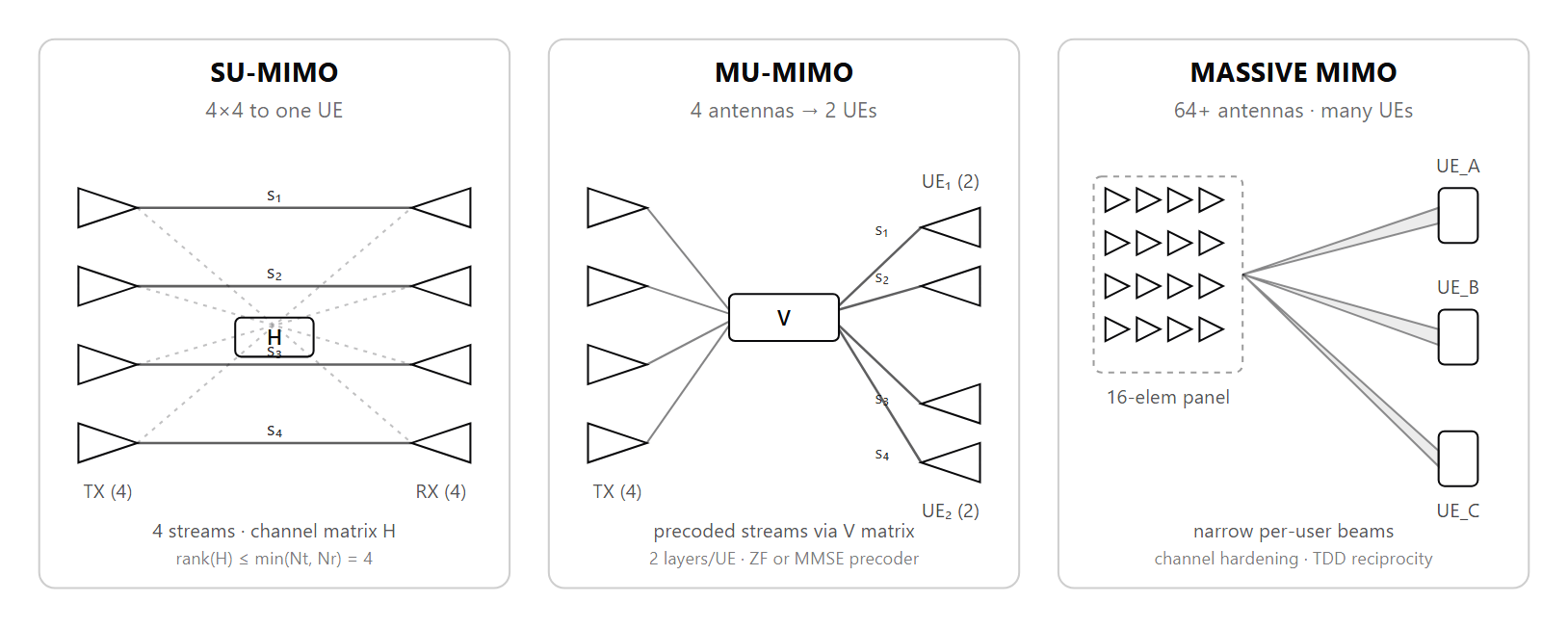
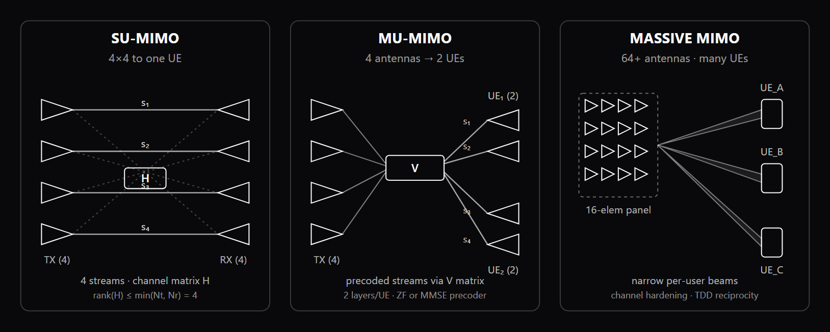
MIMO (Multiple-Input Multiple-Output) is the use of multiple antennas at both the transmitter and receiver to deliver higher spectral efficiency, better link reliability, or both — by exploiting the multiple spatial paths between antenna arrays as independent or correlated channels. The link is described by an Nr × Nt channel matrix H whose entries capture the complex gain between every transmit-receive antenna pair, and the singular value decomposition H = U Σ V^H exposes the parallel eigen-subchannels that set the achievable rate. Standards anchoring: LTE introduced 2x2 baseline MIMO in Rel-8 and scaled to 8x8 SU-MIMO and four-layer MU-MIMO by Rel-13; 5G NR supports up to eight layers per UE on the downlink and arrays up to 256 elements at the gNB for massive-MIMO sub-6 deployments; Wi-Fi 6 standardized 8x8 SU-MIMO and added uplink MU-MIMO for up to 8 users in both directions (Wi-Fi 5/802.11ac was downlink-only, up to 4 users), Wi-Fi 7 doubled the maximum number of spatial streams to 16 (carried on up to a 16×16 antenna array), and Wi-Fi 8 extends coordinated MIMO across access points via Co-BF. The dominant technology stack is the channel matrix H, SVD-based eigenmode precoding with waterfilling for SU-MIMO, ZF and MMSE linear precoders for MU-MIMO co-scheduling, V-BLAST and sphere decoding on the receiver side, and CSI feedback via PMI, CQI, and RI in FDD or TDD reciprocity from SRS sounding in massive-MIMO deployments. Three independent benefits emerge from this structure. Spatial multiplexing sends independent data streams in parallel and scales the link rate by rank(H), which is upper-bounded by min(Nt, Nr) and a function of the multipath richness — sparse-scatterer LOS channels with tight antenna spacing collapse the rank well below the nominal min(Nt, Nr). Spatial diversity transmits the same information across decorrelated paths so that deep fades on any single path do not destroy the message; STBC and SFBC are the canonical implementations. Layer-specific precoding aims energy at a user using the right singular vectors of H, suppressing inter-user interference for co-scheduled UEs and concentrating power where it is needed. Modern systems combine these — a 5G NR gNB might transmit eight layers across two users via Type-II PMI precoding while applying internal coding redundancy per layer. The receiver toolkit ranges from linear MMSE and ZF detection through successive interference cancellation (V-BLAST and MMSE-SIC), sphere decoding, and full maximum-likelihood detection. MU-MIMO extends the framework to multiple co-scheduled users, with the multi-user broadcast-channel sum-capacity achievable in principle by Dirty-Paper Coding and approached in practice by ZF or regularized-ZF precoding. Massive MIMO scales arrays into the dozens-to-hundreds of elements and changes the achievable capacity envelope — channel hardening, near-orthogonal user channels, and pilot contamination all emerge as new operating regimes that conventional 2x2 or 4x4 MIMO never encounters.
Why interviewers ask
MIMO sits at the intersection of linear algebra, communication theory, and practical RF deployment, which makes it a high-leverage interview topic. A wireless or RF candidate who can sketch H, talk through its SVD, and connect that decomposition to the achievable capacity has demonstrated the abstraction muscle the role demands. Interviewers use MIMO questions to test whether you can move between three layers fluently: the math (capacity formulas, SVD-based eigenmode precoding with waterfilling, condition number κ(H) as a rank-stress indicator), the system layer (Type-I vs Type-II PMI codebook tradeoffs in FDD, TDD reciprocity via SRS sounding, MU-MIMO co-scheduling under ZF or regularized-ZF, layer mapping and RI), and the RF reality (how antenna correlation, polarization mismatch, calibration error, and pilot contamination degrade the textbook gains). A favorite probe is asking what limits the rank of a 4x4 outdoor link with strong LOS — candidates who answer "min(4,4) = 4" without flagging the LOS scattering and antenna-spacing constraints flunk the depth check. Another classic is contrasting V-BLAST and MMSE-SIC: candidates who can explain the strongest-first ordering rule, error propagation, and the soft-output coupling to the channel decoder are clearly operating at the level the role needs. MIMO also appears in massive-MIMO contexts where the questions shift to per-element calibration of reciprocity, channel hardening as the array grows, pilot reuse and contamination across cells, and per-user pilot overhead in TDD. Strong candidates connect each topic to a concrete deployment: pilot contamination caps SINR even at M → ∞ because the contaminated channel estimate is applied as a precoder and amplifies the interferer coherently; reciprocity-based MU-MIMO needs continuous over-the-air calibration loops to track per-element TX/RX offsets; Type-II PMI is gated by RRC because its uplink overhead is an order of magnitude larger than Type-I. Sample questions qF8aN3Bz, rH2cT5Wy, sJ6eU1Vp, and uN3iY7Zm cover all three layers.
Common mistakes
Several patterns recur. First, treating MIMO capacity as a fixed multiplier — "4x4 means 4x throughput" — without acknowledging that capacity scales with rank(H) and SNR per stream, not with min(Nt, Nr) alone. Second, conflating spatial multiplexing with spatial diversity: multiplexing transmits independent streams to multiply rate, while diversity sends the same information across decorrelated paths to combat fading. They are different operating points on the same precoding matrix and reward different channel structures. The diversity-multiplexing tradeoff (Zheng-Tse) formalizes the asymptotic exchange. Third, glossing over CSI: a strong candidate distinguishes explicit feedback (FDD codebook PMI like Type-I or Type-II) from implicit feedback (TDD reciprocity from SRS sounding), knows that Type-I quantization caps achievable MU-MIMO gain in FDD, and can explain why TDD reciprocity in massive MIMO collapses to a per-element TX/RX self-calibration problem. Fourth, ignoring the linear-detector-versus-channel-decoder boundary — many candidates describe MMSE detection as if it were the final word, missing that real receivers feed soft information to a turbo or LDPC decoder and that V-BLAST detection ordering, soft-output quality, and iterative cancellation all matter. Fifth, forgetting practical realities: keyhole channels, antenna correlation under tight spacing (see /topics/antenna-design), polarization mismatch, and the per-element TX/RX self-calibration burden that breaks reciprocity in massive-MIMO without active compensation. Strong answers cite a quantitative effect ("rank dropped from 4 to 2 outdoors with 0.5-lambda spacing and dominant LOS") rather than a qualitative one. Reviewers reward that level of specificity. Sixth, missing the multi-cell story. Single-cell MIMO results extrapolate poorly to multi-cell deployments where pilot contamination caps the per-user SINR at a finite asymptote even as the base-station antenna count grows toward infinity. The classical Marzetta result captures this in closed form; the mitigations are coordinated and expensive — pilot reuse factor > 1, time-shifted pilots across cells, large-scale fading decoding, and coordinated joint precoding (JT-CoMP). Candidates who only know the single-cell capacity formulas miss the dominant capacity ceiling in real cellular deployments and undersell the engineering work that goes into operating a massive-MIMO macro cell. Seventh, treating Dirty-Paper Coding as a deployable scheme. DPC is the capacity-achieving non-causal precoder for the multi-user broadcast channel, but it is not implementable in real radios because it assumes non-causal interference knowledge. ZF and regularized-ZF are the practical linear approximations; the gap between ZF sum-rate and DPC sum-capacity converges to a fixed offset at high SNR, and that offset is a function of the spatial correlation across co-scheduled users. Naming DPC precisely as a theoretical bound rather than an implementable algorithm is a strong-candidate signal.
Sample interview questions
- In a 4×4 SU-MIMO link, why does an SVD-based eigenmode precoder with waterfilling outperform equal-power transmission on the four data streams?
- A. SVD diagonalizes H so the receiver can skip channel equalization entirely; equal-power transmission keeps using the linear MMSE detector and therefore pays a fixed 3 dB SNR penalty on every spatial stream that is sent.
- B. SVD compresses the channel matrix into fewer non-zero entries that the transmitter sends back as a quantized PMI; waterfilling is performed by the receiver and re-uses the precoder hardware for the data path.
- C. SVD diagonalizes H = U Σ V^H so the channel splits into parallel eigen-subchannels; waterfilling pours more power into the strong singular values and starves the weakest, maximizing capacity under the total-power constraint. ✓
- D. SVD-based eigenmode precoding doubles the rank of the MIMO channel matrix; waterfilling is just a scaling law and the capacity gain over equal-power comes from the rank increase rather than the power allocation.
Option C is correct because the SVD H = U Σ V^H factors the channel into parallel scalar eigen-subchannels. Right-multiplying the transmit vector by V and left-multiplying the receive vector by U^H decouples the streams into independent AWGN channels with gains equal to the singular values σ_i. Waterfilling solves the constrained capacity problem under total power Σ P_i = P: it pours more power into the eigen-subchannels with large σ_i^2 / N_0 and zero power into the weakest ones when their SNR sits below the water level. The capacity gap over equal-power allocation can be several dB on a poorly-conditioned channel where the smallest σ_i is far below the largest, because equal-power wastes budget on near-noise eigenmodes. Option A is incorrect because SVD-based precoding still needs a per-stream demapper at the receiver — the FFT-style "free equalization" claim is wrong, and equal-power transmission does not pay a fixed 3 dB SNR penalty either. Option B is incorrect because SVD compresses nothing on the wire; the receiver computes SVD on its estimated H, returns a quantized V-matrix index (PMI) for the transmitter to apply, and waterfilling is computed at the transmitter on the reported channel quality indicators, not at the receiver. Option D is incorrect because SVD does not change the rank of H; rank(H) is a fixed property of the channel matrix and SVD just exposes it through the count of non-zero singular values.
- Why does MU-MIMO Zero-Forcing precoding achieve the same high-SNR multiplexing slope as Dirty-Paper Coding, and what residual gap remains under spatial correlation?
- A. ZF achieves DPC capacity exactly at every SNR because both schemes maximize sum-rate under the same total-power constraint; the gap is a textbook artifact of a different normalization convention used in capacity proofs.
- B. ZF outperforms DPC at high SNR because DPC needs non-causal channel knowledge that real radios cannot obtain; the residual gap is a regulatory cap from 3GPP rather than an information-theoretic one for broadcast channels.
- C. ZF detection removes interference but applies to single-user MIMO; the high-SNR capacity gap exists because MU-MIMO must fall back to time-sharing across users instead of co-scheduling them on the same resource block.
- D. ZF nulls inter-user interference but inflates the per-user transmit power as user channels grow correlated; at high SNR the noise term shrinks and the residual ZF penalty converges to a fixed offset versus DPC capacity. ✓
Option D is correct because Zero-Forcing precoding uses the pseudo-inverse of (a regularized form of) the aggregated user channel and transmits along the null spaces of co-scheduled users — interference is removed, but the precoder norm grows as user channels become more colinear, raising the effective per-user noise enhancement. Dirty-Paper Coding (DPC, Costa 1983) achieves the multi-user broadcast-channel sum-capacity by non-causally precoding against known interference; it is information-theoretic and not implementable in real radios. Provided there are enough transmit antennas to serve the co-scheduled users (so the channel is full-rank), the user channels are well-conditioned/near-orthogonal, and the CSIT is accurate and fresh, ZF achieves the same high-SNR multiplexing slope (degrees of freedom) as DPC, but a residual rate/power offset to DPC sum-capacity remains, and that offset grows with the spatial-correlation structure of the user channels. Mitigations include MMSE-regularized ZF (adds σ^2 I to the inverse, the same trick as the MMSE detector), user-pairing heuristics that co-schedule users whose channels are nearly orthogonal, and per-user power loading. Note that ZF detection removes interference at the receiver via the pseudo-inverse — useful in low-noise regimes — but MMSE balances residual interference against amplified noise and is the more robust general-purpose linear scheme. Option A is incorrect because ZF does not match DPC at finite SNR; the multi-user broadcast-channel capacity region is provably strictly larger than the ZF sum-rate, and the difference is not a normalization artifact. Option B is incorrect because ZF does not outperform DPC; DPC is the capacity-achieving non-causal scheme and ZF is a sub-optimal linear approximation. 3GPP rules do not enter the capacity analysis. Option C is incorrect because ZF generalizes naturally to MU-MIMO and is the textbook linear precoder for co-scheduled users; MU-MIMO does not need to fall back to time-sharing when ZF is applied per resource block.
- Why does pilot contamination cap multi-cell massive-MIMO per-user SINR at a finite limit even as the base-station antenna count grows to infinity?
- A. More pilots improve throughput at scale, so adding base-station antennas removes the SINR ceiling once the pilot density exceeds a small threshold; the law of large numbers averages the contamination out across the array elements over time.
- B. Neighboring cells reuse the same uplink pilot sequence, so the channel estimate at one BS is correlated with the interferer in the next cell; the contaminated estimate enters the precoder, and both the desired and interfering coherent gains scale with M antennas, saturating the SINR. ✓
- C. Pilot spacing depends on the delay spread of the channel, so larger arrays automatically pick a coherence-bandwidth-aware pilot pattern that suppresses contamination; the saturation reported in the literature is a transient effect at small M.
- D. Pilot contamination is an FDD impairment driven by quantized PMI feedback; massive-MIMO carriers deployed in TDD avoid it because reciprocity-based sounding does not reuse pilots across neighboring cells in commercial deployments.
Option B is correct because pilot contamination arises when neighboring cells reuse the same orthogonal uplink pilot sequence. The least-squares channel estimate (see /topics/channel-estimation) at base station A becomes a linear combination of the desired user-A channel and the interferer-B channel from the neighboring cell, weighted by the uplink large-scale gains. When this contaminated estimate is then used as the maximum-ratio or ZF precoder for the downlink, the precoder concentrates power not only on user A but also coherently on user B; as the number of base-station antennas M grows, both the desired-signal coherent gain AND the contaminating coherent leakage scale with M, so their ratio (the SINR) converges to a finite asymptote rather than to infinity. The classical Marzetta result quantifies this asymptote in closed form in terms of the pilot-reuse pattern. Mitigations include pilot-reuse factor > 1, time-shifted pilots across cells, large-scale fading decoding, and coordinated joint precoding (JT-CoMP) that treats neighboring cells as cooperative users. Option A is incorrect because more pilots do not improve throughput at scale — increased pilot density reduces spectral efficiency, and the optimal density balances estimation accuracy against pilot overhead. Adding antennas amplifies both the desired and interfering signals jointly; the law of large numbers does not average it out, it scales it up. Option C is incorrect because pilot spacing does not depend solely on delay spread; the frequency spacing depends on coherence bandwidth (and hence delay spread) while the time spacing depends on coherence time (Doppler), and neither choice eliminates the contamination asymptote. Option D is incorrect because pilot contamination is primarily a TDD impairment driven by uplink-sounding-based reciprocity precoding; it has nothing to do with FDD PMI feedback.
- Why does V-BLAST under SIC detect the strongest stream first, and how does the ordering compare to a plain ZF or MMSE linear MIMO detection pass?
- A. Strongest-first ordering is a vendor convention from the V-BLAST receiver datasheet; the ordering does not matter because ZF detection is optimal — it removes inter-stream interference at every SNR — so SIC ordering has no statistical impact on residual SNR.
- B. Strongest-first lets the V-BLAST receiver skip the channel decoder on the strongest stream; subsequent streams reuse the saved decoder cycles to run a larger turbo or LDPC code for higher coding gain on the cleaner residuals.
- C. Strongest-first doubles the receive-antenna spatial degrees of freedom by reusing the antenna array between successive detection passes; this is the central capacity advantage V-BLAST offers over linear ZF or MMSE detection in the wireless literature.
- D. Detecting the strongest stream first minimizes error propagation in the SIC chain; ZF detection removes interference perfectly under a well-conditioned H but amplifies noise at channel nulls, while MMSE balances residual interference against noise. V-BLAST can use ZF or MMSE filters per stage, then adds SIC ordering for extra gain. ✓
Option D is correct because V-BLAST is a successive interference cancellation (SIC) receiver: detect one stream, hard-decide it, subtract its contribution from the received vector, then re-detect the next from the cleaner residual. Cancellation errors propagate down the chain — a wrongly detected symbol leaves a large residual in y, which raises the noise floor for every subsequent stream. The strongest-first rule (detect the stream with highest post-detection SNR first) minimizes head-of-chain error probability and therefore minimizes overall error-propagation impact. The optimal ordering can be derived from the channel pseudo-inverse: detect the stream corresponding to the smallest row norm of (H^H H)^{-1} H^H. The structural contrast with linear detection is that ZF perfectly nulls interference under a well-conditioned channel matrix but amplifies noise at channel nulls because 1/σ_min^2 grows large, while MMSE adds a regularizer to balance residual interference against noise — V-BLAST can be implemented with per-stage ZF or MMSE filtering and layers SIC ordering on top to recover several dB beyond the plain linear detector. Option A is incorrect because the strongest-first rule has rigorous statistical justification — it is provably optimal for minimizing the SER of the first-detected stream and therefore the propagation likelihood; reverse ordering performs measurably worse at high SNR. Option B is incorrect because SIC does not skip the channel decoder; every stream is fully demodulated and decoded. The "saved decoder cycles" argument has no basis in the V-BLAST algorithm. Option C is incorrect because V-BLAST does not change the rank of the received space; the spatial degrees of freedom equal the receive-antenna count regardless of the detection ordering used by the receiver in the SIC chain.
- Why does massive-MIMO favor TDD reciprocity-based sounding over FDD codebook PMI feedback, and what calibration cost does this choice introduce?
- A. TDD reciprocity is mandated by 3GPP for massive-MIMO carriers above 3.5 GHz; FDD codebook PMI is reserved for sub-1-GHz deployments and the per-element calibration question rarely arises at scale in commercial massive-MIMO carriers today.
- B. TDD reciprocity removes the need for downlink demodulation reference signals because the user equipment can derive the precoder from the SRS pattern; the calibration cost is a single factory step and no field calibration is required.
- C. TDD reciprocity replaces per-user PMI feedback (which scales linearly with antennas) with a single SRS that the BS observes on its full array; the cost is per-element TX/RX RF self-calibration to keep the reciprocity assumption valid at hundreds of elements. ✓
- D. TDD reciprocity scales the per-user codebook size exponentially with antenna count, so massive MIMO picks the smallest Type-I codebook to bound feedback overhead; calibration is irrelevant because the feedback path is digital and not analog.
Option C is correct because FDD codebook PMI feedback bandwidth scales with the number of base-station antennas — for a 64-element panel the user equipment must report a high-resolution Type-II PMI on a per-subband cadence, and the uplink overhead alone can consume several percent of cell capacity. TDD reciprocity collapses this to a single SRS transmission per user: the base station observes the uplink channel on its full antenna array and derives the downlink precoder directly, with overhead independent of antenna count. The catch is that the assumed channel reciprocity holds only over the propagation path, not over the radio chains — every transmit chain (DAC → mixer → PA → antenna) and every receive chain (antenna → LNA → mixer → ADC) imposes a per-element phase and amplitude offset that breaks the H_DL = H_UL^T assumption. Massive-MIMO systems therefore add continuous over-the-air self-calibration loops, often by injecting tones through a reference path or by listening to neighboring antennas, to track and compensate per-element offsets across temperature and aging. Option A is incorrect because 3GPP supports both TDD reciprocity and FDD codebook precoding across all bands; the choice is a system-design tradeoff and calibration is a hard engineering problem in practice. Option B is incorrect because downlink demodulation reference signals are still transmitted in TDD reciprocity systems to track residual channel impairments at the user equipment; reciprocity removes PMI feedback but not the DMRS path. Field calibration is also continuous, not one-time. Option D is incorrect because reciprocity does not use codebooks — that is the whole point of the scheme. Codebook size scaling is an FDD problem and irrelevant to the TDD reciprocity tradeoff.
- In 5G NR FDD downlink, why can the Type-II PMI codebook yield higher MU-MIMO sum-rate than the Type-I codebook, and what overhead does it pay?
- A. Type-II PMI is optimal at all SNRs because it reports the best per-layer beam under every channel; the Type-I codebook is reserved for low-SNR conditions where coarser MMSE precoders perform better and ZF precoding at the gNB is also preferred.
- B. Type-II PMI reports a linear combination of multiple DFT beams per layer with amplitude and phase quantization; the higher-resolution precoder unlocks MU-MIMO null-steering, at the cost of uplink feedback roughly an order of magnitude larger than Type-I. ✓
- C. Type-II PMI and Type-I PMI encode the same precoder bits but Type-II adds a CRC field that improves feedback integrity; the capacity gap comes from fewer dropped feedback messages rather than higher-resolution precoder per layer.
- D. Type-II PMI restricts the codebook to SU-MIMO modes and does not support MU-MIMO co-scheduling; the capacity gap is realized in single-user link adaptation and does not appear on the multi-user downlink configurations defined by 3GPP.
Option B is correct because Type-I PMI (Rel-15 baseline) reports one DFT-beam selection per layer plus a coarse per-layer phase — sufficient for SU-MIMO precoding but too coarse for MU-MIMO null-steering. Type-II PMI (Rel-15 enhanced, refined further in Rel-16 with the Type-II port-selection codebook) reports a linear combination of multiple DFT beams per layer with per-coefficient amplitude and phase quantization, giving a much higher-resolution per-user precoder. The richer precoder lets the base station co-schedule users whose channels are nearly orthogonal under the Type-II model and place deep nulls toward the other co-scheduled users; that is what can unlock MU-MIMO sum-rate gains in FDD when the CSI is fresh and the extra feedback overhead is justified — under stale CSI or heavy overhead the net gain can shrink or reverse. The overhead penalty is significant: Type-II feedback bits can be several hundred per CSI report against tens of bits for Type-I, which is why 3GPP gates Type-II by configuration and applies sub-band reporting to amortize the overhead. Option A is incorrect because no PMI codebook is optimal at every SNR — Type-II costs more uplink feedback bits and is gated by RRC configuration on the gNB; for SU-MIMO at moderate channel conditions Type-I is the right pick. ZF and MMSE refer to receive-side and precoding linear schemes, not to PMI codebook selection rules. Option C is incorrect because Type-I and Type-II do not encode the same precoder bits; they are fundamentally different codebook structures and a CRC field is not the source of the capacity gap. Option D is incorrect because Type-II PMI is explicitly designed for MU-MIMO co-scheduling; the MU-MIMO gain is the primary motivation for the higher-resolution feedback path on the downlink.
- Why does high UE mobility erode the gain of closed-loop PMI-based precoded MIMO, and what precoding behavior is more robust when CSI feedback goes stale?
- A. High mobility keeps the PMI fresh because faster fading is averaged out over the CSI reporting window, so closed-loop precoding actually gains array directivity as UE speed increases.
- B. High mobility is irrelevant to closed-loop precoding because the precoder is recomputed at the UE every slot from downlink reference signals, so feedback latency never enters the loop.
- C. High mobility only affects HARQ retransmissions, not precoding; the gNB always precodes from the most recent PMI and the channel-aging effect is fully removed by RI reporting at a slower cadence.
- D. When the channel decorrelates faster than the CSI reporting cadence, the reported PMI is stale by the time it is applied, so the precoder is matched to an out-of-date channel and the closed-loop array gain collapses; a feedback-independent precoder (e.g. precoder cycling / large-delay CDD that spreads each layer across many precoders) is more robust because it collects diversity without trusting an instantaneous PMI. ✓
Option D is correct because closed-loop precoded MIMO depends on the PMI/CQI/RI report being a fresh snapshot of the channel. When the user equipment moves fast (vehicular or high-speed-rail UEs) the channel coherence time falls below the CSI reporting and feedback-delay budget, so the gNB ends up precoding for a channel state that no longer holds — the constructive array gain is lost and can even turn destructive. A feedback-independent strategy is more robust: a deterministic precoder-cycling pattern (large-delay cyclic delay diversity in LTE, precoder cycling more generally) spreads each layer across many precoders over time and frequency, so the link collects diversity without trusting an instantaneous PMI. Rank is still reported (rank indicator, RI) at a slower cadence, but the per-resource precoder no longer relies on a fresh per-slot PMI. The trade is reduced beamforming/array gain in exchange for robustness to channel aging. Option A is incorrect because faster fading does not keep PMI fresh; shorter coherence time makes the report stale sooner, which degrades — not improves — closed-loop precoding. Option B is incorrect because closed-loop precoding is computed at the gNB from UE-reported PMI, so feedback latency and channel aging absolutely enter the loop; the UE does not recompute and apply the downlink precoder itself. Option C is incorrect because channel aging hits the precoder directly, not just HARQ; RI is reported at a slower cadence and does not undo a stale per-slot PMI.
Frequently asked questions
- What is the difference between spatial multiplexing and spatial diversity?
- Spatial multiplexing sends independent data streams in parallel over multiple antenna pairs to multiply throughput; the achievable number of streams is bounded by the rank of the MIMO channel matrix H, which depends on the richness of the multipath. Spatial diversity sends the same information across multiple antennas to combat fading; gain comes from the probability that not all paths fade simultaneously. Multiplexing buys peak throughput when SNR is high and rank is large; diversity buys reliability when SNR is low or H is poorly conditioned. Real systems mix both — for example, a 4x4 MIMO link might transmit two streams (multiplexing) while applying space-time coding (STBC or SFBC) within each stream (diversity). The diversity-multiplexing tradeoff (Zheng-Tse 2003) formalizes the asymptotic exchange between the two regimes. Sample question wR8mC6Eh drills into how the closed-loop precoded multiplexing mode falls back to open-loop cycling when channel feedback becomes stale on a fast-moving UE.
- What is channel rank and why does it cap MIMO throughput?
- Channel rank is the number of linearly independent eigenmodes of H at a given time and frequency — equivalently, the count of non-zero singular values in the SVD H = U Σ V^H. The number of usable parallel streams is upper-bounded by min(Nt, Nr, rank(H)). Rank can fall below min(Nt, Nr) when scatterers are sparse (line-of-sight without rich multipath), antenna spacing is too small (correlated channels), or the receiver is in a keyhole-like geometry where the entire array sees the propagation environment through a narrow pinch-point. A nominal 4x4 link can collapse to rank 1 outdoors with strong LOS and tight antenna spacing, which is why MU-MIMO with co-scheduled users — each contributing additional spatial degrees of freedom — often outperforms single-user spatial multiplexing in real deployments. Rank-adaptive scheduling (RI feedback per CSI report) is standard in LTE and 5G NR and is reported separately from PMI.
- How do MMSE and ZF MIMO detectors differ?
- Zero-Forcing inverts the channel matrix to decouple streams: x_hat = (H^H H)^{-1} H^H y. It cleanly separates streams when H is well-conditioned, but at low SNR or near-singular H the pseudo-inverse amplifies noise catastrophically because (H^H H)^{-1} has large eigenvalues — the noise enhancement term grows as 1/σ_min^2 where σ_min is the smallest singular value of H. MMSE adds a regularizer proportional to the noise variance: x_hat = (H^H H + σ^2 I)^{-1} H^H y. The result balances residual inter-stream interference against amplified noise, giving graceful degradation at low SNR and a tighter post-detection SNR. MMSE is the de facto industrial baseline; ZF tends to appear in textbooks and in special cases where H is provably well-conditioned and computational simplicity matters. The two converge at high SNR (σ^2 → 0) but diverge sharply when the channel condition number κ(H) is large. Sample question rH2cT5Wy contrasts ZF/MMSE precoding against the DPC capacity bound on the multi-user downlink.
- What is V-BLAST and how does it improve over linear MIMO detection?
- V-BLAST (Vertical Bell Labs Layered Space-Time) is a successive interference cancellation receiver: detect the strongest stream first, subtract its contribution from the received vector, then re-detect the next strongest from the cleaner residual, and so on. The strongest-first ordering matters because cancellation errors propagate down the SIC chain, so the rule limits damage by minimizing the error probability of the head-of-chain decision. Compared to linear MMSE, V-BLAST trades a small increase in latency and complexity for several dB of SNR gain when the channel is reasonably stationary. Modern implementations couple V-BLAST with soft-output cancellation (feeding soft symbols instead of hard decisions into the next stage), sphere decoding inside the SIC loop, and turbo iterations with the channel decoder to extract more of the capacity. Pure ML detection is the upper bound; V-BLAST is one of the most popular near-ML approaches. Sample question tL9gW4Xk probes the strongest-first ordering rule.
- What is the difference between explicit and implicit CSI feedback?
- Explicit CSI feedback transmits a quantized representation of H or its eigenvectors back to the transmitter; the gNB or AP then designs a precoder using full channel knowledge. Implicit feedback assumes channel reciprocity (typically TDD): the receiver transmits sounding pilots (SRS in 5G NR uplink), the base station measures them on the uplink, and the precoder is computed from the local estimate without any quantization. Explicit feedback works in FDD where reciprocity does not hold and supports codebook-based precoders like 3GPP Type-I and Type-II PMI, but consumes uplink overhead and quantizes the channel; implicit feedback eliminates the feedback channel but requires precise self-calibration of TX/RX RF chains across the array so the reciprocity assumption actually holds. NR supports both modes; massive MIMO at sub-6 leans heavily on TDD reciprocity. Sample question uN3iY7Zm covers the calibration cost; sample question vP5kA2Bd contrasts Type-I and Type-II PMI overhead.
- How does massive MIMO differ from conventional MIMO?
- Conventional MIMO uses a handful of antennas at each end (2x2, 4x4, 8x8) and treats spatial dimensions explicitly per user. Massive MIMO scales the base-station array to dozens or hundreds of elements, far more than the number of simultaneously served UEs. With many more BS antennas than active users, the channels of different users become approximately orthogonal under favorable propagation, which lets simple linear precoders (matched filter, ZF, MMSE) approach the multi-user capacity. Massive MIMO also enables narrow user-specific layer mapping, dramatic interference suppression, and 3D precoding that exploits the elevation dimension. Channel hardening is another consequence: the per-user channel norm concentrates around its mean as the array grows, so fast fading on the data path effectively disappears. The cost is calibration: hundreds of RF chains have to be amplitude- and phase-aligned for reciprocity-based MU-MIMO to work, and pilot contamination caps SINR at a finite asymptote even with M → ∞ antennas. Sample question sJ6eU1Vp drills into pilot contamination.
- How does the 5G NR Type-I PMI codebook compare to Type-II at the resource-allocation layer?
- Type-I PMI (Rel-15 baseline) reports a single best DFT beam per layer with coarse per-layer phase quantization — sufficient for SU-MIMO precoding and inexpensive in feedback bits, but too coarse for MU-MIMO co-scheduling because the resulting precoder cannot reliably null toward other scheduled users. Type-II PMI (Rel-15 enhanced, with refinements in Rel-16 including the Type-II port-selection codebook) reports a linear combination of multiple DFT beams per layer with per-coefficient amplitude and phase quantization, giving a much higher-resolution per-user precoder. The richer precoder lets the gNB co-schedule users whose channels are nearly orthogonal under the Type-II model and place deep nulls toward the other co-scheduled users; that is what unlocks MU-MIMO sum-rate gains in FDD. The cost is uplink overhead — Type-II feedback bits can be roughly an order of magnitude larger than Type-I per CSI report, which is why 3GPP gates Type-II by RRC configuration and applies sub-band reporting to amortize the cost across the carrier. Sample question vP5kA2Bd quantifies the tradeoff.
- What is the difference between open-loop and closed-loop spatial multiplexing in 5G NR?
- Closed-loop spatial multiplexing reports a fresh PMI/CQI/RI per CSI period and the gNB adapts the precoder on every slot to the latest channel snapshot. This maximizes array gain when the channel is stable — low-mobility stationary UEs or static indoor deployments — but degrades when the channel decorrelates faster than the reporting cadence, because the precoder applied at the slot is no longer matched to the current H. Open-loop spatial multiplexing transmits a deterministic cycled precoder across layers and resource blocks (large-delay CDD in LTE, precoder cycling in NR transmission scheme tx-config) so the system collects diversity across layers without depending on instantaneous channel feedback. Rank is still reported via RI at a slower cadence, but the per-slot precoder is fixed. The right operating point depends on UE speed and channel coherence: high-mobility vehicular UEs favor open-loop because PMI staleness would erase closed-loop gains; low-mobility static UEs favor closed-loop because the feedback stays fresh. Sample question wR8mC6Eh drills into when each mode wins.
- How does Wi-Fi spatial-stream support evolve from 802.11ac through 802.11bn, and why does 16x16 sounding cost matter?
- IEEE 802.11ac (Wi-Fi 5) standardized up to 8 spatial streams with explicit NDP-based beamforming sounding and compressed PMI feedback. 802.11ax (Wi-Fi 6) kept the 8-stream cap and added uplink MU-MIMO. 802.11be (Wi-Fi 7) doubled the maximum number of spatial streams from 8 to 16 — which requires up to a 16×16 antenna configuration, since the stream count can never exceed min(Tx, Rx) antennas (a spatial stream is an independent data stream, not an antenna pair) — the capability behind the headline EHT peak rate, though real clients implement far fewer. It also added Multi-Link Operation so a Multi-Link Device can carry independent streams across affiliated links on 2.4, 5, and 6 GHz simultaneously — see /topics/multi-link-operation-deep-dive for the MLO mechanism details. 802.11bn (Wi-Fi 8) does not raise the stream count further; it targets ultra-high reliability — worst-case latency, tail throughput, and multi-AP coordination. The dominant practical cost of sounding a 16-Tx × 16-Rx channel (the configuration Wi-Fi 7 enabled) is airtime: the Null Data Packet must carry training fields for each transmit stream, the receiver must estimate a 16-column channel matrix, and the compressed beamforming feedback frame grows proportionally. The sounding cadence bounds how fast the channel can be re-sounded under mobility, which directly affects MU-MIMO scheduling and rate adaptation. See /topics/wifi-8 sample question fO8qY2Bs for a deeper drill into the 16x16 sounding tradeoff.
- How does NR beam management apply MIMO principles in FR2?
- At FR2 (24+ GHz), NR uses analog and hybrid beamforming (see /topics/beamforming) with narrow beams, and the architecture adds explicit beam-management procedures: P-1 (initial beam acquisition via SSB sweep), P-2 (gNB Tx beam refinement via CSI-RS), P-3 (UE Rx beam refinement via CSI-RS). The TCI-state framework binds each scheduled transmission to a source reference signal with a QCL relationship; QCL Type-D specifically conveys the spatial-RX beam configuration, the FR2-critical addition. See /topics/nr-beam-management for the full beam-management procedure layer and the QCL type details.
Related topics
Pillar
Siblings
- Wireless Foundations
- Beamforming Interview Guide: Analog vs Digital vs Hybrid
- OFDM Explained: Subcarriers, Cyclic Prefix, PAPR, and OFDMA
- Antenna Design
- DSP Fundamentals
- Channel Estimation
- LTE-Advanced
- 5G NR Explained: Numerology, BWP, HARQ, and Frame Structure
- Linear Algebra
- NR Reference Signals: DMRS, CSI-RS, SRS, PTRS, and the SSB
Practice
Essential AI-Native Skills for MIMO Explained: Spatial Multiplexing, Rank, Massive MIMO
Modern engineering work increasingly uses AI tools for design and code review, debugging, documentation, test and testbench generation, and workflow automation. The goal is not to let AI replace engineering judgment — it is to move faster while keeping verification discipline.
- Use AI to explain unfamiliar code, logs, waveforms, datasheets, or test failures.
- Break large problems into small, reviewable steps you can verify independently.
- Ask AI for hypotheses, then validate them against tests, measurements, simulations, or lab data.
- Version-control your analysis scripts, testbenches, and configs — keep changes small and reviewable.
- Document your assumptions, design tradeoffs, and debugging decisions.
- Verify AI output before trusting it: run the checks that fit the domain — unit tests, linters, simulations, or bench/lab measurements.
- Review AI output for correctness, edge cases, and real-world consequences.